1. Lecture 8 Magnetopause Magnetosheath Bow shock Fore Shock Homework: 6

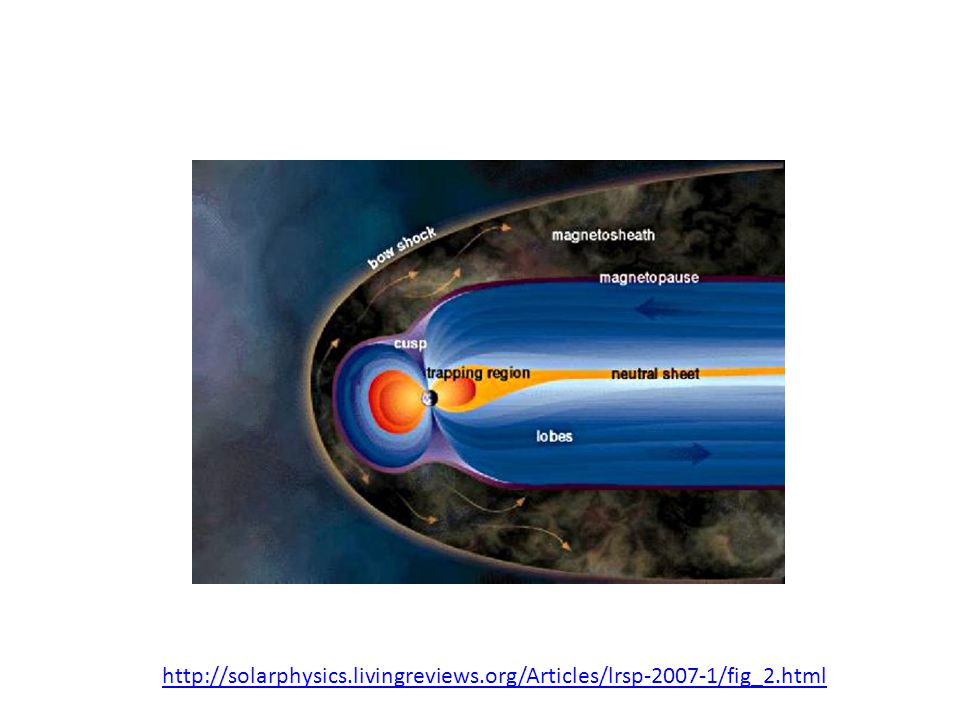
2. http://solarphysics. livingreviews. org/Articles/lrsp-2007-1/fig_2

3. Outline Earth’s Dipole Field Solar Wind at 1 AU Bow Shock
Magnetosheath
Magnetopause

4. Earth’s Dipole Field Components
To a first approximation the magnetic field of the Earth can be expressed a that of the dipole. The dipole moment of the Earth is tilted ~110 to the rotation axis with a present day value of 8·1015 Tm3 or 30.4·10-6 TRE3 where RE=6371 km (one Earth radius).
In a coordinate system fixed to this dipole moment where θ is the magnetic colatitude, and M is the dipole magnetic moment.
The dipole moment of the Earth presently is ~8·1015T m3 (3·10-5TRE3 ).

5. Earth’s Dipole Field Lines
Magnetic field lines are everywhere tangent to the magnetic field vector.
Integrating r= r0sin2θ where r0 is the distance to equatorial crossing of the field line.
It is most common to use the magnetic latitude λ instead of the colatitude
r= Lcos2 λ
where L is measured in RE.
Equation of a field line:

6. Earth’s Dipole Axis and Moment
The dipole moment of the Earth presently is ~8·1015T m3 (3·10-5TRE3).
The dipole moment is decreasing.
9.5·1015T m3 in 1550
7.84·1015T m3 in 1990.
The dipole moment is tilted ~110 with respect to the rotation axis. The tilt is changing.
30 in 1550
11.50 in 1850
10.80 in 1990.
In addition to the tilt angle the rotation axis of the Earth is inclined by with respect to the ecliptic pole.
Thus the Earth’s dipole axis can be inclined by ~350 to the ecliptic pole.
The angle between the direction of the dipole and the solar wind varies between 560 and 900.

7. Earth’s Dipole Field

8. Solar Wind at 1 AU Time Period: 1963-1986
Two complete sunspot cycles (20+21)
Spacecraft
IMP-1
IMP-2
IMP-8
AIMP-1
AIMP-2
OGO-5
HEOS
VELA-1 to -6
ISEE-1 to -3
Hapgood, M. A., et al. (1991) Variability of the interplanetary medium at 1 AU over 24 years: , Planet. Space Sci., 39, 3, pp

9. For example, IMP-8 IMP J (IMP 8, Interplanetary Monitoring Platform-J)
IMP 8 Description
Launch Date:  On-orbit dry mass:  kg Nominal Power Output:  W IMP 8 (Explorer 50), the last satellite of the IMP series, is a drum-shaped spacecraft, cm across and cm high, instrumented for interplanetary and magnetotail studies of cosmic rays, energetic solar particles, plasma, and electric and magnetic fields. Its initial orbit was more elliptical than intended, with apogee and perigee distances of about 45 and 25 RE. Its eccentricity decreased after launch. Its orbital inclination varied between 0° and about 55° with a periodicity of several years. The spacecraft spin axis was normal to the ecliptic plane, and the spin rate was 23 rpm. The spacecraft was in the solar wind for 7 to 8 days of every 12.5 day orbit. The objectives of the extended IMP-8 operations were to provide solar wind parameters as input for magnetospheric studies and as a 1-AU baseline for deep space studies, and to continue solar cycle variation studies with a single set of well-calibrated and understood instruments.

10. For example: ISEE-3
ISEE-3 originally operated in a halo orbit about the L1 Sun-Earth Lagrangian point, 235 Earth radii above the surface (about 1.5 million km, or 924,000 miles). It was the first artificial object placed at a so-called "libration point", proving that such a suspension between gravitational fields was possible.
The purposes of the mission were:
to investigate solar-terrestrial relationships at the outermost boundaries of the Earth's magnetosphere;
to examine in detail the structure of the solar wind near the Earth and the shock wave that forms the interface between the solar wind and Earth's magnetosphere;
to investigate motions of and mechanisms operating in the plasma sheets; and,
to continue the investigation of cosmic rays and solar flare emissions in the interplanetary region near 1 AU.

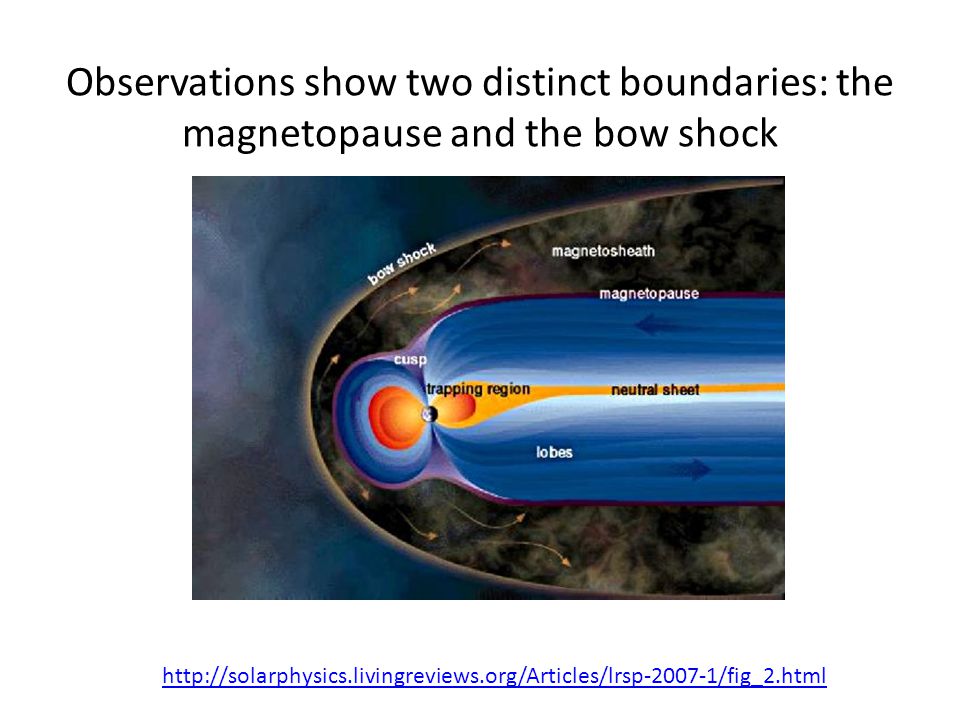
11. Observations show two distinct boundaries: the magnetopause and the bow shock

12. Distortion of Earth’s Field

13. Observations show two distinct boundaries: the magnetopause and the bow shock

14. Working Definition of Earth’s Bow Shock
“Earth's bow shock represents the outermost boundary between that region of geospace which is influenced by Earth's magnetic field and the largely undisturbed interplanetary medium streaming from the Sun.”

15. Bow Shock and Magnetopause Crossings
Song

16. Bow Shock Crossings with Location Front Orientation
Song

17. Solar Wind Driver
The Bow Shock is the interface between Earth’s magnetic field and the Solar Wind.
The Earth’s magnetic field is distorted by the Solar Wind.
A sheath is formed.
What are the aspects of the Solar Wind that create the Bow Shock?

18. Solar Wind at 1 AU
Field flips every cycle (opposite polarity in successive cycles)
Sun’s Field Reversal Near Solar Maximum
Highest Velocities when phase is declining
<|Bz|> is highest around Solar Maximum
Hapgood, M. A., et al. (1991) Variability of the interplanetary medium at 1 AU over 24 years: , Planet. Space Sci., 39, 3, pp

19. Solar Wind Near 1 AU

20. Solar Wind Near 1 AU

21. Solar Wind Energetics Solar Wind Energy From
Magnetic Field
Thermal Properties of Particles
Flow (Dynamic Pressure)
Which component has the highest energy density?

22. Solar Wind Energy Densities at 1 AU
Also recall:
Average
Alfvén Mach
Number
Average
Sound Mach
Number

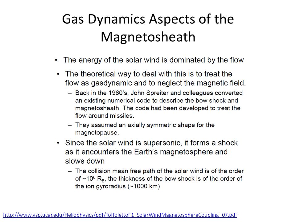
23. Gas Dynamics Aspects of the Magnetosheath

24. Stream Lines

25. Bow shock and magnetosheath divert the solar wind flow around the magnetosphere: computer simulation
Song

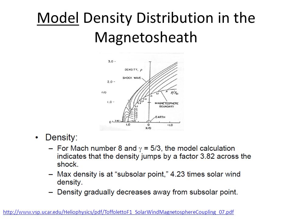
26. Model Density Distribution in the Magnetosheath

27. Observations of Density Enhancements in the Sheath
Song

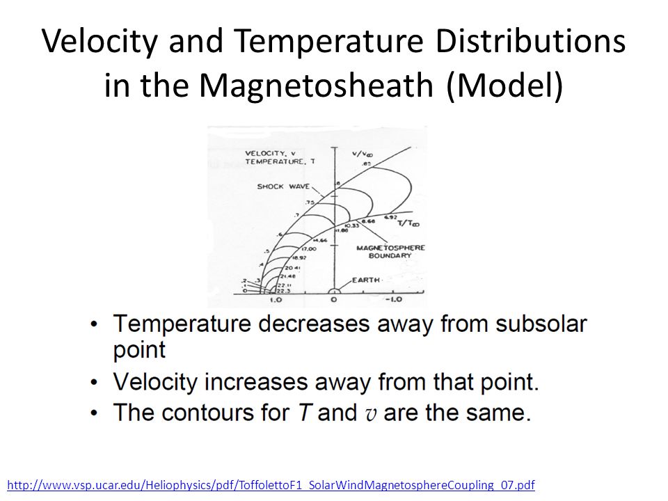
28. Velocity and Temperature Distributions in the Magnetosheath (Model)

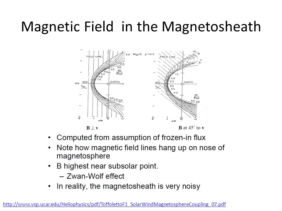
29. Magnetic Field in the Magnetosheath

30. Effects of Mach Number

31. Observations of β vs. Alfvén Mach Number
Collisionless Shocks
1) Subcritical: dissipation is due to dispersion and/or anomalous resistivity
2) Supercritical: ambient plasma conditions require additional processes to dissipate energy including ion reflection and large amplitude plasma waves
Winterhalter and Kivelson, (1988) Observations of the Earth's Bow Shock Under High Mach Number/High Plasma Beta Solar Wind Conditions, GRL, 15, 10, pp

32. Formation of Sonic Shock

33. Formation of a Standing Shock Front
Song

34. Definition of a Shock Song
A shock is a discontinuity separating two different regimes in a continuous media.
Shocks form when velocities exceed the signal speed in the medium.
A shock front separates the Mach cone of a supersonic jet from the undisturbed air.
Characteristics of a shock :
The disturbance propagates faster than the signal speed. In gas the signal speed is the speed of sound, in space plasmas the signal speeds are the MHD wave speeds.
At the shock front the properties of the medium change abruptly. In a hydrodynamic shock, the pressure and density increase while in a MHD shock the plasma density and magnetic field strength increase.
Behind a shock front a transition back to the undisturbed medium must occur. Behind a gas-dynamic shock, density and pressure decrease, behind a MHD shock the plasma density and magnetic field strength decrease. If the decrease is fast a reverse shock occurs.
A shock can be thought of as a non-linear wave propagating faster than the signal speed.
Information can be transferred by a propagating disturbance.
Shocks can be from a blast wave - waves generated in the corona.
Shocks can be driven by an object moving faster than the speed of sound.
Song

35. Shock Frame of Reference
The Shock’s Rest Frame
In a frame moving with the shock the gas with the larger speed is on the left and gas with a smaller speed is on the right.
At the shock front irreversible processes lead the the compression of the gas and a change in speed.
The low-entropy upstream side has high velocity.
The high-entropy downstream side has smaller velocity.
Collisionless Shock Waves
In a gas-dynamic shock collisions provide the required dissipation.
In space plasmas the shocks are collision free.
Microscopic Kinetic effects provide the dissipation.
The magnetic field acts as a coupling device.
MHD can be used to show how the bulk parameters change across the shock.
Shock Front
Upstream
(low entropy)
Downstream
(high entropy) vu vd
Song

36. Shock Conservation Laws
In both fluid dynamics and MHD conservation equations for mass, energy and momentum have the form: where Q and are the density and flux of the conserved quantity.
If the shock is steady ( ) and one-dimensional or that
where u and d refer to upstream and downstream and is the unit normal to the shock surface. We normally write this as a jump condition
Conservation of Mass or If the shock slows the plasma then the plasma density increases.
Conservation of Momentum where the first term is the rate of change of momentum and the second and third terms are the gradients of the gas and magnetic pressure in the normal direction.
Song

37. Conservation of energy
Conservation of momentum The subscript t refers to components that are transverse to the shock (i.e. parallel to the shock surface).
Conservation of energy
The first two terms are the flux of kinetic energy (flow energy and internal energy) while the last two terms come form the electromagnetic energy flux
Gauss Law gives
Faraday’s Law gives
Song

38. Types of Discontinuities in Ideal MHD
The jump conditions are a set of 6 equations. If we want to find the downstream quantities given the upstream quantities then there are 6 unknowns ( ρ ,vn,,vt,,p,Bn,Bt).
The solutions to these equations are not necessarily shocks. These conservations laws and a multitude of other discontinuities can also be described by these equations.
Types of Discontinuities in Ideal MHD
Contact Discontinuity ,
Density jumps arbitrary, all others continuous. No plasma flow. Both sides flow together at vt.
Tangential Discontinuity
Complete separation. Plasma pressure and field change arbitrarily, but pressure balance
Rotational Discontinuity
Large amplitude intermediate wave, field and flow change direction but not magnitude.
Song

39. Types of Shocks in Ideal MHD
Shock Waves
Flow crosses surface of discontinuity accompanied by compression.
Parallel Shock
B unchanged by shock.
Perpendicular Shock
P and B increase at shock
Oblique Shocks
Fast Shock
P, and B increase, B bends away from normal
Slow Shock
P increases, B decreases, B bends toward normal.
Intermediate Shock
B rotates 1800 in shock plane, density jump in anisotropic case
Song

40. Configuration of magnetic field lines for fast and slow shocks
Configuration of magnetic field lines for fast and slow shocks. The lines are closer together for a fast shock, indicating that the field strength increases. [From Burgess, 1995].
Song

41. Functions of Magnetosheath
Diverts the solar wind flow and bends the IMF around the magnetopause
Song

42. Internal Structure of the Magnetosheath
Bow Shock
Magnetopause
Post-bow shock density
Song

43. Slow Shock in the Magnetosheath
Song

44. Foreshock
The first particles observed behind the tangent line are electrons with the highest energy electrons closest to the tangent line – electron foreshock.
A similar region for ions is found farther downstream – ion foreshock.
Particles can be accelerated in the shock (ions to 100’s of keV and electrons to 10’s of keV).
Some can leak out and if they have sufficiently high energies they can out run the shock. (This is a unique property of collisionless shocks.)
At Earth the interplanetary magnetic field has an angle to the Sun-Earth line of about 450. The first field line to touch the shock is the tangent field line.
At the tangent line the angle between the shock normal and the IMF is 900.
Lines further downstream have
Particles have parallel motion along the field line ( ) and cross field drift motion ( ).
All particles have the same
The most energetic particles will move farther from the shock before they drift the same distance as less energetic particles
Song

45. Ion Foreshock
Song

46. Upstream Waves

47. Summary of Foreshock: shock-field angle determines the features in the sheath and upstream
Song

48. There are shocks in structures/entities in the S/W.
These shocks also interact with the Earth’s Magnetosphere.
They are associated with IMF conditions that cause
Geomagnetic Storms. Geomagnetic Substorms are related to
Processes that return flux that is transported to the tail back
To the dayside.
We’ve talked about the solar wind. The next slides
Explain how to find shocks in the solar wind.

49. Shocks in the Solar Wind
Solar Wind has entities/events like Coronal Mass Ejections (CME) and Corrotating Interaction Regions (CIR)
CME are associated with magnetic clouds and have shocks and sheaths
CIR have shocks
The interaction of CME/CIR and Earth’s magnetosphere results in a geomagnetic storm driven by these shocks and southward IMF.

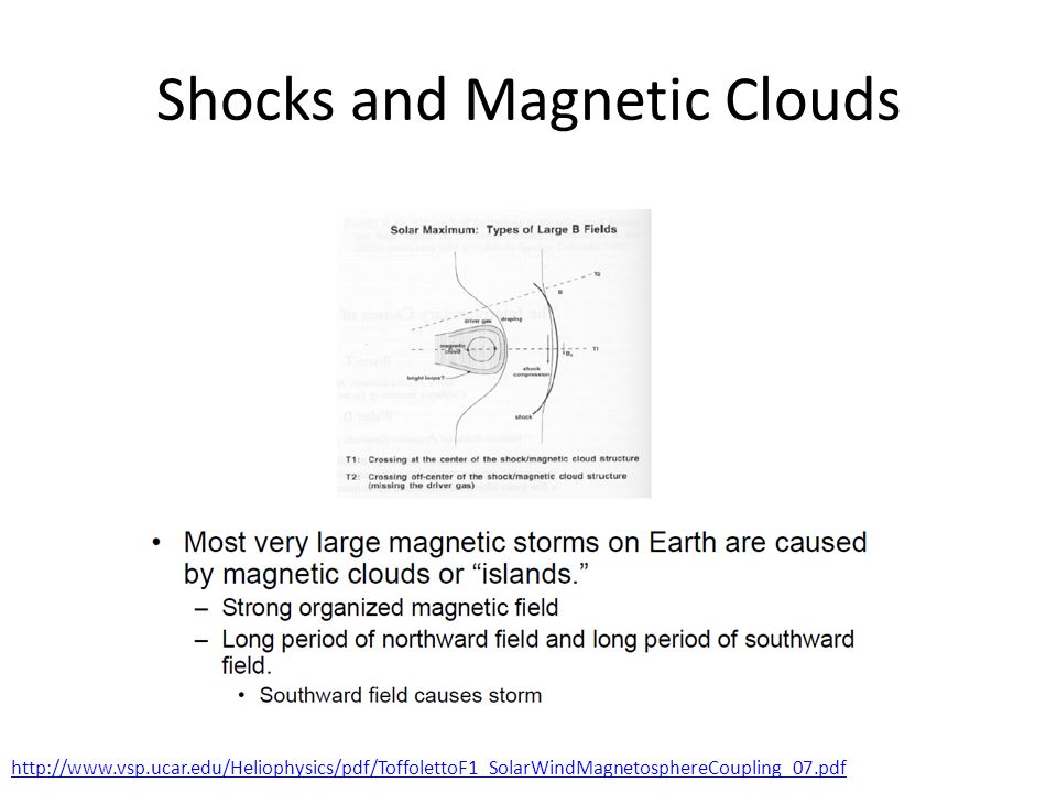
50. Shocks and Magnetic Clouds

51. Case Study CME Solar Wind at 1 AU Zhang CME 3/19 1154
V=860km/s
Angular Width=180° (partial halo is ≥120°, halo is 360°)
M1.0Flare
AR9866 S10W58
producing a SH(M)+ICME(M)
Shock arrival at 3/23/11:24 (inferred from Wind)
ICME 3/ to 3/ Class 2
CME 3/
V=603km/s AW=180d
AR9871 S21W15
Zhang CME 3/
Shock arrival at 3/23/11:24 (inferred from Wind)
ICME 3/ to 3/ Class 2 (1AU)
Jian ICME (1AU Wind)
‘Hybrid event’ (not only one event)
ICME 3/ to 3/
Start of Magnetic Obstacle 3/
Discontinuity 3/ Forward Shock
Ptmax=180 pPa, Vmax=490(520) km/s , Vmin=410 km/s, Bmax=21nT, Group=1
2/ F
Comments: Vp irregular, followed by an SIR
Group 1: central maximum of Pt
Group 2: plateau-like profile of Pt
Group 3: gradual decrease after sharp
increase of leading edge.
Jian, L., et. al. (2006) Properties of interplanetary coronal mass ejections at one AU during , Solar Physics, 239, pp. 393–436
DOI: /s
Zhang, J., et. al. (2007) Solar and interplanetary sources of major geomagnetic storms (Dst <= -100 nT) during , JGR, 112, A10102, pp. 1-19, doi: /2007JA012321

52. Shock Noah Jian Shocks:
8-Hz magnetic field data – rotated into shock normal coordinates to examine the existence of associated shock waves and field changes consistent with R-H relations
Forward shock: all of Vs, Np, Tp, and magnetic field should increase simultaneously.
Reverse shocks: Vs increases while Np, Tp, and magnetic field all decrease.
Not all shocks have clear signatures in plasma properties.
Noah

53. SUN  CME  ICME  SYMH Reconnection drives convection
Convection drives the ring current.
Midlatitude ground magnetometers H component decreases.
Worldwide stations make SYMH

54. Shock

55. IMF Crosses the Bow Shock
Southward IMF crosses into the sheath region and merges/reconnects with the Earth’s magnetic field at the magnetopause.
The formation of the magneotpause is the next topic.
Chapter 8 AFRL Handbook of Geophysics, 1985

56. Showed the beginning of the reconnection
Slides to explain how the solar wind IMF interacts
With the Magnetopause and the Convection cycle.
The following slides were after a blackboard
Drawing explaining the 3 topologies of magnetic field:
Open with both footprints in the S/W
Open with one footprint in S/W and one on Earth
Closed with both footprints on Earth
So, it was explained that Maxwell’s equations require no
‘open’ field lines, they all have to close, but locally we
Regard these lines as ‘open’ although we know they
Terminate on the Sun or Heliopause, local to Earth that
Is not important for understanding Magnetosphere processes.

57. Solar Wind-Magnetosphere Interaction: Reconnection and IMF Dependence

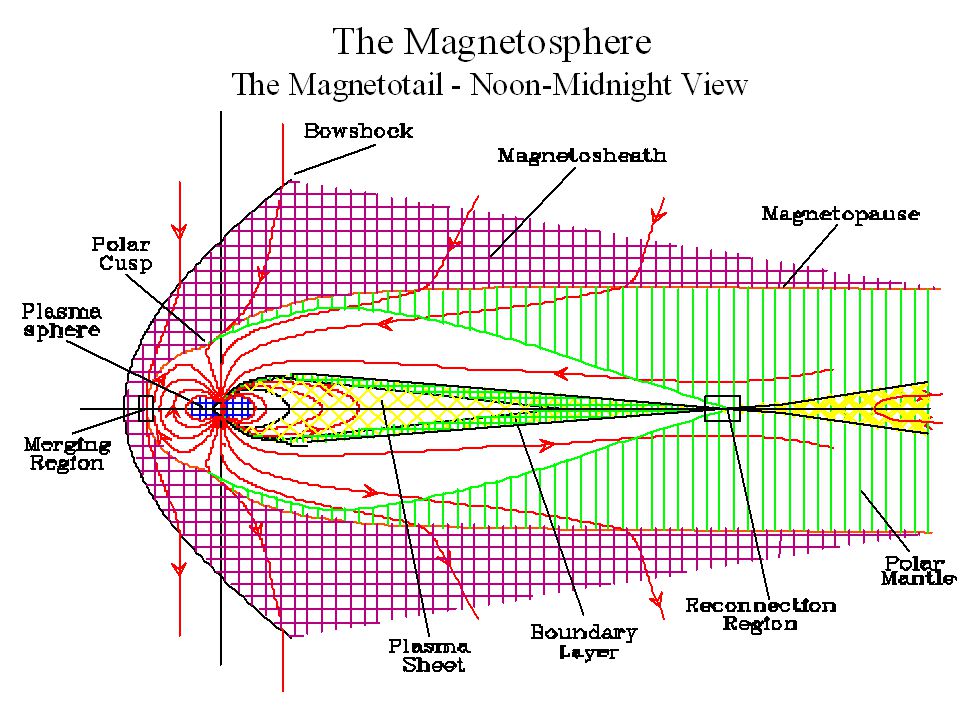
60. The Magnetosphere The Magnetotail
The magnetotail is the region of the magnetosphere that stretches away from the Sun behind the Earth.
It acts as a reservoir for plasma and energy. Energy and plasma from the tail are released into the inner magnetosphere a periodically during magnetospheric substorms.
A current sheet lies in the middle of the tail and separates it into two regions called the lobes.
The magnetic field in the north (south)lobe is directed away from (toward) the Earth.
The magnetic field strength is typically ~20 nT.
Plasma densities are low (<0.1 cm-3). Very few particles in the 5-50keV range. Cool ions observed flowing away from the Earth with ionospheric composition. The tail lobes normally lie on “open” magnetic field lines.

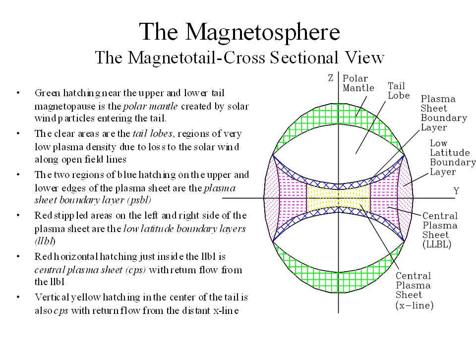
62. The Magnetosphere The Magnetotail - Structure
The plasma mantle has a gradual transition from magnetosheath to lobe plasma values.
Flow is always tailward
Flow speed, density and temperature all decrease away from the magnetopause.
Ions in the plasma sheet boundary layer (PSBL) typically flow at 100s of km/s parallel or antiparallel to the magnetic field.
Frequently counterstreaming beams are observed: one flowing earthward and one flowing tailward.
Densities are typically 0.1 cm-3.
The PSBL is thought to be on “closed” magnetic field lines.
The central plasma sheet (CPS) consists of hot (kilovolt) particles that have nearly symmetric velocity distributions.
Typical densities are 0.1-1cm-3 with flow velocities that the small compared to the ion thermal velocity (the electron temperature is 1/7 of the ion temperature).
The CPS is usually on “closed” field lines but can be on “plasmoid” field lines.

63. The Magnetosphere The Magnetotail - Structure Continued
The low latitude boundary layer (LLBL) contains a mix of magnetosheath and magnetospheric plasma.
Plasma flows can be found in almost any direction but are generally intermediate between the magnetosheath flow and magnetospheric flows.
The LLBL extends from the dayside just within the magnetopause along the flanks of the magnetosphere forming a boundary between the plasma sheet and the magnetosheath.
Note there is a region in the tail where the plasma mantle, PSBL and LLBL all come together.
The origins of the plasma mantle and the plasma sheet boundary layer are clear but the origin of the low latitude boundary layer is less clear.

64. The Magnetotail - Typical Plasma and Field Parameters
The Magnetosphere
The Magnetotail - Typical Plasma and Field Parameters

65. The Magnetosphere ReconnectionZ X

66. The Magnetosphere Reconnection
As long as frozen in flux holds plasmas can mix along flux tubes but not across them.
When two plasma regimes interact a thin boundary will separate the plasma
The magnetic field on either side of the boundary will be tangential to the boundary (e.g. a current sheet forms).
If the conductivity is finite and there is no flow Faraday’s law and Ampere’s law give a diffusion equation
Magnetic field diffuses down the field gradient toward the central plane where it annihilates with oppositely directed flux diffusing from the other side.
This reduces the field gradient and the whole process stops but not until magnetic field energy has been converted into heat via Joule heating (the resulting pressure increase is what is needed to balance the decrease in magnetic field pressure).

67. The Magnetosphere Reconnection Continued
For the process to continue flow must transport magnetic flux toward the boundary at the rate at which it is being annihilated.
An electric field in the Ey ( ) direction will provide this in flow.
In the center of the current sheet B=0 and Ohm’s law gives
If the current sheet has a thickness 2l Ampere’s law gives
Thus the current sheet thickness adjusts to produce a balance between diffusion and convection. This means we have very thin current sheets.
There is no way for the plasma to escape this system. If the diffusion is limited in extent then flows can move the plasma out through the sides.

68. The Magnetosphere Reconnection Continued
When the diffusion is limited in space annihilation is replaced by reconnection
Field lines flow into the diffusion region from the top and bottom
Instead of being annihilated the field lines move out the sides.
In the process they are “cut” and “reconnected” to different partners.
Plasma originally on different flux tubes, coming from different places finds itself on a single flux tube in violation of frozen in flux.
The boundary which originally had Bx only now has Bz as well.
Reconnection allows previously unconnected regions to exchange plasma and hence mass, energy and momentum.
Although MHD breaks down in the diffusion region, plasma is accelerated in the convection region where MHD is still valid.

69. The Magnetosphere Reconnection
Acceleration due to slow shocks
Emanating from the diffusion region are four shock waves indicated by dashed lines (labeled separatrix).
At the shocks the magnetic field and flow change abruptly.
The magnetic field strength decreases
The flow speed increase but the normal flow decreases.
These structures are current sheets. The flow is accelerated by the
force.

70. The Magnetosphere Reconnection
By the 1950’s it was realized that plasma flows observed in the polar and auroral ionospheres must be driven by magnetospheric flows.
Flow in the polar regions was from noon toward midnight.
Return flow toward the Sun was at somewhat lower latitudes.
This flow pattern is called magnetospheric convection.
If all flux tubes remained within the magnetosphere then the flow pattern is like that in a falling rain drop caused by viscous effects.
Dungey in 1961 showed that if magnetic field lines reconnected in front of the magnetosphere the required pattern would result.

71. The Magnetosphere Reconnection
When IMF Bz driven by the solar -wind flow against the dayside magnetopause is southward reconnection occurs between field lines 1 (closed with both ends at the Earth) and the IMF field line 1’
This forms two new field lines with one end at the Earth and one end in the solar wind (called open).
The solar wind will pull its end tailward ( )
In the ionosphere this will drive flow tailward as observed.
If this process continued indefinitely without returning some flux the Earth’s field would be lost.
Another neutral line is needed in the tail.