1. A Flexible Bayesian Method to Model Adverse Event Hazards Quan Hong, Scott Andersen, Dave DeBrota Midwest Biopharmaceutical Statistics Workshop May 19, 2009

2. Value Proposition Model Adverse Event Hazard Rate Identify risk factors –such as patient gender, ethnicity, or age Or rule them out –E.g., not because of dosing duration. Applicable even when N is small (N = 30 or 40), or n is small (n = 3 or 5)

3. Motivational Example Preclinical animal toxicology studies Animals were given different dosages : 50mg/kg, 100mg/kg …, 300 mg/kg Animals were dosed once a day for 3 months, 6 months or 1 year. 5 – 10 animals per dose group Some animals had an emisis in higher dose group, while others did not through the duration of the studies

4. A Red dot indicates an animal having an emesis 2 dogs (out of 10) on 300mg/kg had events on day 2 and 10 2 dogs (out of 8) on 200mg/kg had events on day 30 and 60 1 dog (out of 14) on 100mg/kg had an event on day 200 and 300

5. Was emesis due to increased doses? Was emesis due to longer dosing duration? Motivational Example (Cont’d)

6. Modeling

7. Poisson distribution expresses the probability of a number of events occurring in a fixed period of time if these events occur with a known average rate and independently of the time since the last event. Number of events Average event rate

8. Day 1Day 2Day d How many emeses did the dog have on day 1? How many emeses did the dog had on day 2? on day d?

9. is the average rate of adverse events rate of patient i on day d If AE rate is related to dosing duration (days), If AE rate is also related to daily dosage (mg), a and b are model parameters is the number of adverse events a patient i had on day d, then follows Poisson distribution, where Model Put Bayesian priors on a and b,

10. a, the dose coefficient If a > 0 Dose If a = 0 More AEs at higher doses AEs evenly across doses If a < 0 Not likely!

11. b, the time coefficient If b > 0 Time Increased AE frequency with time If b = 0 Time AEs evenly across time If b < 0 Time Decreasing AE frequency with time

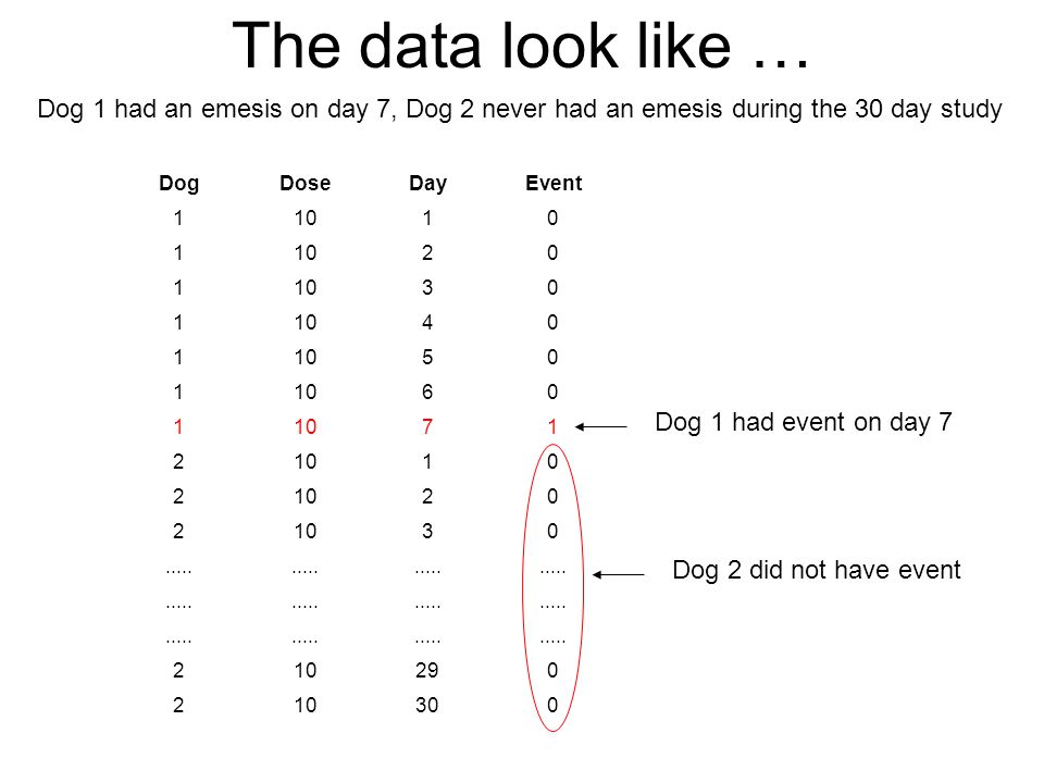
12. The data look like … Dog 1 had an emesis on day 7, Dog 2 never had an emesis during the 30 day study Dog 1 had event on day 7 Dog 2 did not have event DogDoseDayEvent 11010 1 20 1 30 1 40 1 50 1 60 1 71 2 10 2 20 2 30..... 210290 210300

13. Apply the Model in WinBUGS or R/BRugs model { for ( i in 1 : N){ response[i] ~ dpois(lambda[i]) lambda[i] <- a * doses[i] + b * times[i] } a ~ dnorm(0,4.0E4) b ~ dnorm(0,4.0E4) }

14. Simulation Flow Diagram Step 1 : Select pre-specified a and b, N (# of dogs), and T (duration of study) -e.g., a = 0.0005, b = 0.00001 Step 2 : Simulate a dataset according to selected and Step 3 : Apply the model to get a and b estimators Step 4 : Repeat steps 2 and 3 for M times, e.g (M = 1000), and get M sets of estimators and Step 5 : Assess the simulation results of 1000 sets of estimators for precision and bias

15. Simulation

16. Simulation Scenario I – “N” is small a = 0.0005, b = 0.0001 3 dose groups : 10, 20 and 50 mg/kg N = 10 / group Typical simulated dataset shown below

18. Simulation Scenario II – “n” is small a = 0.0001, b = 0 3 dose groups : 10, 20 and 50 mg/kg N = 10 / group Typical simulated dataset is shown below

19. Simulation Scenario II

20. Case Examples

21. Example I (Preclinical) – Motivational Example

22. Example I - Results

23. Example I - conclusion Dog emesis rate increases with dose Dog emesis rate does not change with time

24. Example II – Olanzapine Long- Acting Injection Post-injection syndrome (29 events in 41,193 injections) Previously identified risk factors –Logistic regression –Dose –Age –BMI Also interested in question of constant hazard

25. Example II - WinBUGS Model model { for ( i in 1 : 41193){ eventyn[i] ~ dpois(lambda2[i]) lambda[i] <- b0 +b1 * bmi[i] + b2 * age[i] + b3 * sdydose[i] + b4 * injno[i] lambda2[i]<-max(lambda[i],0.00001) } b0 ~ dnorm(0,6.25E6) b1 ~ dnorm(0,6.25E6) b2 ~ dnorm(0,6.25E6) b3 ~ dnorm(0,6.25E6) b4 ~ dnorm(0,6.25E6) }

26. Example II - Results

27. Example II - conclusion Previously identified risk factors were significant Hazard rate does not increase over time Hazard for a specific patient –age = 50 –BMI = 22 –dose = 405mg –0.0019 (logistic regression calculated as 0.0022)

28. Flexibility The Poisson probabilistic part of the model Can be replaced with other distributions and models as determined by different problems, for example :

29. Concluding Remarks AE hazard rate modeling –Works well even when N is small or n is small –Applies to a wide variety of data : preclinical, clinical or market data Risk factors –Identify risk factors, or rule them out. –Address toxicity or safety concerns early and effectively. Flexibility –May use different distributions, different priors or different hazard rate functions depending on situation –Easy to implement using WinBUGS or R/BRugs