1. FOURIER SERIES Philip Hall Jan 2011
Definition of a Fourier series
A Fourier series may be defined as an expansion of a function in a series
of sines and cosines such as
(7.1)
The coefficients are related to the periodic function f(x)
by definite integrals: Eq.(7.11) and (7.12) to be mentioned later on.
Henceforth we assume f satisfies the following (Dirichlet) conditions:
(1) f(x) is a periodic function;
(2) f(x) has only a finite number of finite discontinuities;
(3) f(x) has only a finite number of extrem values, maxima and minima in the
interval [0,2p].
Fourier series are named in honour of Joseph Fourier ( ), who made important contributions to the study of trigonometric series, in connection with the solution of the heat equation

2. (7.3)
Expressing cos nx and sin nx in exponential form, we may rewrite Eq.(7.1) as
(7.4)
in which
(7.5)
and
(7.6)

3. Completeness and orthogonality
We can show Fourier series satisfy
certain completeness properties- see next year
Now we need to find out how to determine the coefficients
in the Fourier series expansion and find out in what circumstances the
Fourier series and function coincide..

4. We can easily check the orthogonal relation for different values of the eigenvalue n by
choosing the interval
(7.7)
(7.8)
for all integer m and n.
(7.9)

5. By use of these orthogonality, we are able to obtain the coefficients
(7.9)
Similarly
(7.10)
(7.11)
(7.12)
Substituting them into Eq.(7.1), we write

6. EXAMPLE: Sawtooth wave
(7.13)
This equation offers one approach to the development of the Fourier integral and
Fourier transforms.
EXAMPLE: Sawtooth wave
Let us consider a sawtooth wave
(7.14)
For convenience, we shall shift our interval from to
. In this interval
we have simply f(x)=x. Using Eqs.(7.11) and (7.12), we have

7. So, the expansion of f(x) reads
(7.15) .
Figure 7.1 shows f(x) for the sum of 4, 6, and 10 terms of the series.
Three features deserve comment.
There is a steady increase in the accuracy of the representation as the number of
terms included is increased.
2.All the curves pass through the midpoint at

8. Figure 7.1 Fourier representation of sawtooth wave

9. CONVERGENCE OF FOURIER SERIES
W assume f satisfies the following (Dirichlet) conditions:
(1) f(x) is a periodic function;
(2) f(x) has only a finite number of finite discontinuities;
(3) f(x) has only a finite number of extrem values, maxima and minima in the
interval [0,2p].
We can then show that at a point where f(x) is
continuous the Fourier series converges to f(x). However
at a point of discontinuity the Fourier series converges to
½(sum of right and left hand limits of limits of f(x). Hence at any point x
(7.18)
where of course the right and left hand limits coincide where f is continuous.

10. 7.2 ADVANTAGES, USES OF FOURIER SERIES
Discontinuous Function
One of the advantages of a Fourier representation over some other representation,
such as a Taylor series, is that it may represent a discontinuous function. An example
id the sawtooth wave in the preceding section. Other examples are considered in
Section 7.3 and in the exercises.
Periodic Functions
Related to this advantage is the usefulness of a Fourier series representing a periodic
functions . If f(x) has a period of
, perhaps it is only natural that we expand it in ,
a series of functions with period , ,
This guarantees that if
our periodic f(x) is represented over one interval or
the
representation holds for all finite x.

11. is an even function of x. Hence ,
At this point we may conveniently consider the properties of symmetry. Using the
interval ,
is odd and
is an even function of x. Hence ,
by Eqs. (7.11) and (7.12), if f(x) is odd, all
if f(x) is even all
. In
other words,
even, (7.21)
odd (7.21)
Frequently these properties are helpful in expanding a given function.
We have noted that the Fourier series periodic. This is important in considering
whether Eq. (7.1) holds outside the initial interval. Suppose we are given only that
(7.23)
and are asked to represent f(x) by a series expansion. Let us take three of the
infinite number of possible expansions.

12. 1.If we assume a Taylor expansion, we have
(7.24)
a one-term series. This (one-term) series is defined for all finite x.
2.Using the Fourier cosine series (Eq. (7.21)) we predict that
(7.25)
3.Finally, from the Fourier sine series (Eq. (7.22)), we have
(7.26)

13. Figure 7.2 Comparison of Fourier cosine series, Fourier sine series and Taylor series.

14. These three possibilities, Taylor series, Fouries cosine series, and Fourier sine series,
are each perfectly valid in the original interval
. Outside, however, their behavior
is strikingly different (compare Fig. 7.3). Which of the three, then, is correct? This
question has no answer, unless we are given more information about f(x). It may be
any of the three ot none of them. Our Fourier expansions are valid over the basic
interval. Unless the function f(x) is known to be periodic with a period equal to our
basic interval, or
th of our basic interval, there is no assurance whatever that
representation (Eq. (7.1)) will have any meaning outside the basic interval.
It should be noted that the set of functions ,
, forms a
complete orthogonal set over
. Similarly, the set of functions ,
forms a complete orthogonal set over the same interval. Unless forced
by boundary
conditions or a symmetry restriction, the choice of which set to use is arbitrary.

15. FOURIER SERIES OVER ARBITRARY INTERVALS
So far attention has been restricted to an interval of length of
. This restriction
may easily be relaxed. If f(x) is periodic with a period
, we may write
(7.27)
with
(7.28)
(7.29)

16. replacing x in Eq. (7.1) with
and t in Eq. (7.11) and (7.12) with
(For convenience the interval in Eqs. (7.11) and (7.12) is shifted to
. )
The choice of the symmetric interval (-L, L) is not essential. For f(x) periodic with
a period of 2L, any interval
will do. The choice is a matter of
convenience or literally personal preference.

17. HALF RANGE FOURIER SERIES
We have seen above that even and odd functions have Fourier series
With either or zero.
Now suppose we have a function defined on an interval [0,K], then
we extend it as an even or odd function of period K so as to produce a Fourier
cosine or sine series. But note the period is now 2K, it is always wise
to sketch the extended function.
Exercise: extend the functions given below as odd and even functions,
sketch the extended functions and give the formulae for the Fourier coefficients:
(7.4-5)
Note that extending a function to produce either an odd or even function
can lead to discontinuities.

18. 7.3 APPLICATION OF FOURIER SERIES)
7.3 APPLICATION OF FOURIER SERIES
Example Square Wave ——High Frequency
One simple application of Fourier series, the analysis of a “square” wave (Fig. (7.5))
in terms of its Fourier components, may occur in electronic circuits designed to
handle sharply rising pulses. Suppose that our wave is designed by

19. (7.30)
From Eqs. (7.11) and (7.12) we find
(7.31)
(7.32)
(7.33)

20. Example 7.3.2 Full Wave Rectifier
The resulting series is
(7.36)
Except for the first term which represents an average of f(x) over the interval
all the cosine terms have vanished. Since
is odd, we have a Fourier sine
series. Although only the odd terms in the sine series occur, they fall only as
This is similar to the convergence (or lack of convergence ) of harmonic series.
Physically this means that our square wave contains a lot of high-frequency
components. If the electronic apparatus will not pass these components, our square
wave input will emerge more or less rounded off, perhaps as an amorphous blob.
Example Full Wave Rectifier
As a second example, let us ask how the output of a full wave rectifier approaches
pure direct current (Fig. 7.6). Our rectifier may be thought of as having passed the
positive peaks of an incoming sine and inverting the negative peaks. This yields

21. Since f(t) defined here is even, no terms of the form will appear.
(7.37)
Since f(t) defined here is even, no terms of the form
will appear.
Again, from Eqs. (7.11) and (7.12), we have
(7.38)

22. is not an orthogonality interval for both sines and cosines
(7.39)
Note carefully that
is not an orthogonality interval for both sines and cosines
together and we do not get zero for even n. The resulting series is
(7.40)
The original frequency
has been eliminated. The lowest frequency oscillation is
The high-frequency components fall off as
, showing that the full wave
rectifier does a fairly good job of approximating direct current. Whether this good
approximation is adequate depends on the particular application. If the remaining ac components are objectionable, they may be further suppressed by appropriate filter circuits.

23. These two examples bring out two features characteristic of Fourier expansion.
1. If f(x) has discontinuities (as in the square wave in Example 7.3.1), we can expect
the nth coefficient to be decreasing as
. Convergence is relatively slow.
If f(x) is continuous (although possibly with discontinuous derivatives as in the
Full wave rectifier of example 7.3.2), we can expect the nth coefficient to be
decreasing as
3. More generally if f and its first r derivatives are continuous, but the r+1 is not
then the nth coefficient will be decreasing as
Example Infinite Series, Riemann Zeta Function
As a final example, we consider the purely mathematical problem of
expanding
(7.41)

24. by symmetry all
For the
’s we have
(7.42)
(7.43)
From this we obtain
(7.44)

25. As it stands, Eq. (7.44) is of no particular importance, but if we set
(7.45)
and Eq. (7.44) becomes
(7.46) or
(7.47)
thus yielding the Riemann zeta function,
, in closed form. From our
expansion of
and expansions of other powers of x numerous other
infinite series can be evaluated.

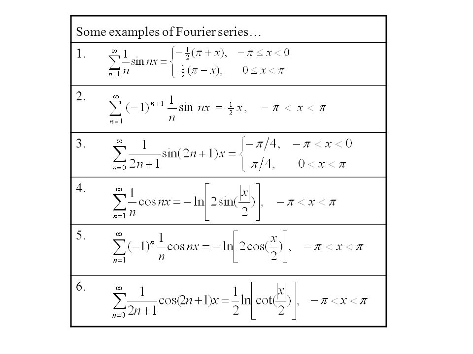
26. Some examples of Fourier series…1. 2. 3. 4. 5. 6.

27. 7.4 Properties of Fourier Series
Convergence
It might be noted, first that our Fourier series should not be expected to be
uniformly convergent if it represents a discontinuous function. A uniformly
convergent series of continuous function (sinnx, cosnx) always yields a continuous
function. If, however,
(a) f(x) is continuous,
(b)
(c)
is sectionally continuous,
the Fourier series for f(x) will converge uniformly. These restrictions do not demand
that f(x) be periodic, but they will satisfied by continuous, differentiable, periodic
function (period of )

28. Integration
Term-by-term integration of the series
(7.60)
yields
(7.61)
Clearly, the effect of integration is to place an additional power of n in the
denominator of each coefficient. This results in more rapid convergence than
before. Consequently, a convergent Fourier series may always be integrated
term by term, the resulting series converging uniformly to the integral of the
original function. Indeed, term-by-term integration may be valid even if the
original series (Eq. (7.60)) is not itself convergent! The function f(x) need only
be integrable.

29. Strictly speaking, Eq. (7.61) may be a Fourier series; that is , if
there will be a term
. However,
(7.62)
will still be a Fourier series.
Differentiation
The situation regarding differentiation is quite different from that of integration.
Here thee word is caution. Consider the series for
(7.63)
We readily find that the Fourier series is
(7.64)

30. Differentiating term by term, we obtain
(7.65)
which is not convergent ! Warning. Check your derivative
For a triangular wave which the convergence is more rapid (and uniform)
(7.66)
Differentiating term by term
(7.67)

31. which is the Fourier expansion of a square wave
(7.68)
As the inverse of integration, the operation of differentiation has placed an
additional factor n in the numerator of each term. This reduces the rate of
convergence and may, as in the first case mentioned, render the differentiated
series divergent.
In general, term-by-term differentiation is permissible under the same conditions
listed for uniform convergence.

32. COMPLEX FORM OF FOURIER SERIES
Recall from earlier that we can write a Fourier series in the complex form
in which
and
From the earlier definitions of we can show that

33. The multiplication theorem and Parsevals theorem
From the complex form of the definition of Fourier series for functions
f(x), g(x) of period 2T we can show that
Where the c,d’s are the Fourier coefficients of f,g respectively.
If we use the repalce the c’d’s by their real form and take f=g
we deduce Paresevals theorem , ,