COMP5331: Knowledge Discovery and Data Mining

COMP5331: Knowledge Discovery and Data Mining
Acknowledgement: Slides modified by Dr. Lei Chen based on the slides provided by Jiawei Han, Micheline Kamber, and Jian Pei ©2012 Han, Kamber & Pei. All rights reserved. 1 1

Chapter 9. Classification: Advanced Methods
Classification by Backpropagation Support Vector Machines Additional Topics Regarding Classification Summary 2 2

Biological Neural Systems
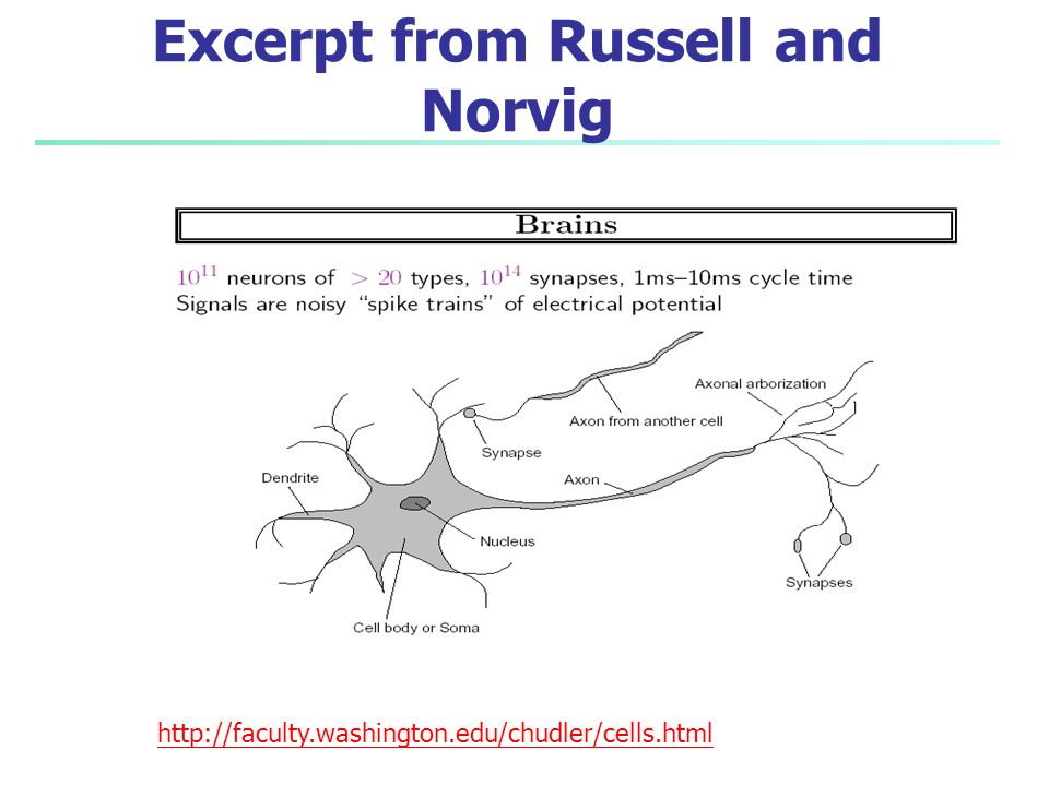
Neuron switching time : > 10-3 secs Number of neurons in the human brain: ~1010 Connections (synapses) per neuron : ~104–105 Face recognition : 0.1 secs High degree of distributed and parallel computation Highly fault tolerent Highly efficient Learning is key

Excerpt from Russell and Norvig

Modeling A Neuron on Computer
xi Wi output y Input links output links å y = output(a) Computation: input signals  input function(linear)  activation function(nonlinear)  output signal

Part 1. Perceptrons: Simple NN
inputs weights x1 w1 output activation w2 x2  y . q a=i=1n wi xi wn xn Xi’s range: [0, 1] 1 if a  q y= 0 if a < q {

To be learned: Wi and q 1 1 Decision line w1 x1 + w2 x2 = q x2 w 1 x1
x1 1

Converting To (1) (2) (3) (4) (5)

{  . Threshold as Weight: W0 a= i=0n wi xi x0=-1 x1 w1 w0 =q w2 x2 y
wn 1 if a  0 y= 0 if a <0 { xn

{ Linear Separability a= i=0n wi xi 1 if a  0 y= 0 if a <0 x1 x2
q=1.5 1 x1 a= i=0n wi xi 1 if a  0 y= 0 if a <0 { Logical AND x1 x2 a y -1.5 1 -0.5 0.5 t 1

XOR cannot be separated!
Logical XOR w1=? w2=? q= ? x1 x2 t 1 1 x1 1 Thus, one level neural network can only learn linear functions (straight lines)

Training the Perceptron
Training set S of examples {x,t} x is an input vector and T the desired target vector (Teacher) Example: Logical And Iterative process Present a training example x , compute network output y , compare output y with target t, adjust weights and thresholds Learning rule Specifies how to change the weights W of the network as a function of the inputs x, output Y and target t. x1 x2 t 1

Perceptron Learning Rule
wi := wi + Dwi = wi + a (t-y) xi (i=1..n) The parameter a is called the learning rate. In Han’s book it is lower case L It determines the magnitude of weight updates Dwi . If the output is correct (t=y) the weights are not changed (Dwi =0). If the output is incorrect (t  y) the weights wi are changed such that the output of the Perceptron for the new weights w’i is closer/further to the input xi.

Perceptron Training Algorithm
Repeat for each training vector pair (x,t) evaluate the output y when x is the input if yt then form a new weight vector w’ according to w’=w + a (t-y) x else do nothing end if end for Until fixed number of iterations; or error less than a predefined value a: set by the user; typically = 0.01

Example: Learning the AND Function : Step 1.
W0 W1 W2 0.5 x1 x2 t 1 a=(-1)*0.5+0*0.5+0*0.5=-0.5, Thus, y=0. Correct. No need to change W a: = 0.1

1 W0 W1 W2 0.5 a=(-1)*0.5+0* *0.5=0, Thus, y=1. t=0, Wrong. DW0= 0.1*(0-1)*(-1)=0.1, DW1= 0.1*(0-1)*(0)=0 DW2= 0.1*(0-1)*(1)=-0.1 a: = 0.1 W0= =0.6 W1=0.5+0=0.5 W2= =0.4

1 W0 W1 W2 0.6 0.5 0.4 a=(-1)*0.6+1* *0.4=-0.1, Thus, y=0. t=0, Correct! a: = 0.1

1 W0 W1 W2 0.6 0.5 0.4 a=(-1)*0.6+1* *0.4=0.3, Thus, y=1. t=1, Correct a: = 0.1

{ Final Solution: a= 0.5x1+0.4*x2 -0.6 1 if a  0 y= 0 if a <0 x1
w1=0.5 w2=0.4 w0=0.6 1 x1 a= 0.5x1+0.4*x2 -0.6 1 if a  0 y= 0 if a <0 { Logical AND x1 x2 1 y 1

Perceptron Convergence Theorem
The algorithm converges to the correct classification if the training data is linearly separable and learning rate is sufficiently small (Rosenblatt 1962). The final weights in the solution w is not unique: there are many possible lines to separate the two classes.

Experiments

Handwritten Recognition Example

Each letter  one output unit y
x1 w1 w2 x2  . wn xn weights (trained) fixed Input pattern Association units Summation Threshold

Multiple Output Perceptrons
Handwritten alphabetic character recognition 26 classes : A,B,C…,Z First output unit distinguishes between “A”s and “non-A”s, second output unit between “B”s and “non-B”s etc. . . . y1 y2 y26 wji connects xi with yj . . . x1 x2 x3 xn w’ji = wji + a (tj-yj) xi

Part 2. Multi Layer Networks
Output vector Output nodes Hidden nodes Input nodes Input vector

Sigmoid-Function for Continuous Output
inputs weights x1 w1 output activation w2 x2  O . a=i=0n wi xi wn xn O =1/(1+e-a) Output between 0 and 1 (when a = negative infinity, O = 0; when a= positive infinity, O=1.

Gradient Descent Learning Rule
For each training example X, Let O be the output (bewteen 0 and 1) Let T be the correct target value Continuous output O a= w1 x1 + … + wn xn + O =1/(1+e-a) Train the wi’s such that they minimize the squared error E[w1,…,wn] = ½ kD (Tk-Ok)2 where D is the set of training examples

Explanation: Gradient Descent Learning Rule
Ok wi xi wi = a Ok (1-Ok) (Tk-Ok) xik activation of pre-synaptic neuron learning rate error dk of post-synaptic neuron derivative of activation function

Backpropagation Algorithm (Han, Figure 9.5)
Initialize each wi to some small random value Until the termination condition is met, Do For each training example <(x1,…xn),t> Do Input the instance (x1,…,xn) to the network and compute the network outputs Ok For each output unit k Errk=Ok(1-Ok)(tk-Ok) For each hidden unit h Errh=Oh(1-Oh) k wh,k Errk For each network weight wi,j Do wi,j=wi,j+wi,j where wi,j= a Errj* Oi, θj=θj+θj where θj = a Errj, a: is learning rate, set by the user;

Multilayer Neural Network
Given the following neural network with initialized weights as in the picture(next page), we are trying to distinguish between nails and screws and an example of training tuples is as follows: T1{0.6, 0.1, nail} T2{0.2, 0.3, screw} Let the learning rate (l) be 0.1. Do the forward propagation of the signals in the network using T1 as input, then perform the back propagation of the error. Show the changes of the weights. Given the new updated weights with T1, use T2 as input, show whether the predication is correct or not.

Answer: First, use T1 as input and then perform the back propagation. At Unit 3: a3 =x1w13 +x2w23+θ3 =0.14 o3 = = 0.535 Similarly, at Unit 4,5,6: a4 = 0.22, o4 = 0.555 a5 = 0.64, o5 = 0.655 a6 = , o6 = 0.534

Now go back, perform the back propagation, starts at Unit 6: Err6 = o6 (1- o6) (t- o6) = * ( )*( ) = 0.116 ∆w36 = (l) Err6 O3 = 0.1 * * = w36 = w36 + ∆w36 = ∆w46 = (l) Err6 O4 = 0.1 * * = w46 = w46 + ∆w46 = ∆w56 = (l) Err6 O5 = 0.1 * * = w56 = w56 + ∆w56 = θ6 = θ6 + (l) Err6 = * =

Continue back propagation: Error at Unit 3: Err3 = o3 (1- o3) (w36 Err6) = * ( ) * (-0.394*0.116) = w13 = w13 + ∆w13 = w13 + (l) Err3X1 = *( ) * 0.6 = w23 = w23 + ∆w23 = w23 + (l) Err3X2 = *( ) * 0.1 = θ3 = θ3 + (l) Err3 = * ( ) = Error at Unit 4: Err4 = o4 (1- o4) (w46 Err6) = * ( ) * ( *0.116) = 0.003 w14 = w14 + ∆w14 = w14 + (l) Err4X1 = *(-0.003) * 0.6 = w24 = w24 + ∆w24 = w24 + (l) Err4X2 = *(-0.003) * 0.1 = θ4 = θ4 + (l) Err4 = * (0.003) = Error at Unit 5: Err5 = o5 (1- o5) (w56 Err6) = * ( ) * ( *0.116) = 0.016 w15 = w15 + ∆w15 = w15 + (l) Err5X1 = * * 0.6 = w25 = w25 + ∆w25 = w25 + (l) Err5X2 = *0.016 * 0.1 = θ5= θ5 + (l) Err5 = * =

After T1, the updated values are as follows: Now, with the updated values, use T2 as input: At Unit 3: a3 = x1w13 + x2w23 + θ3 = o3 = = 0.515

Similarly, a4 = , o4 = 0.565 a5 = , o5 = At Unit 6: a6 = x3w36 + x4w46 + x5w56 + θ6 = o6 = = Since O6 is closer to 1, so the prediction should be nail, different from given “screw”. So this predication is NOT correct.

Example 6.9 (HK book, page 333) X1 1 4 Output: y X2 6 2 5 X3 3
Eight weights to be learned: Wij: W14, W15, … W46, W56, …, and q Training example: x1 x2 x3 t 1 Learning rate: =0.9

Initial Weights: randomly assigned (HK: Tables 7.3, 7.4)
x1 x2 x3 w14 w15 w24 w25 w34 w35 w46 w56 q4 q5 q6 1 0.2 -0.3 0.4 0.1 -0.5 -0.2 -0.4 Net input at unit 4: Output at unit 4:

Feed Forward: (Table 7.4) Continuing for units 5, 6 we get:
Output at unit 6 = 0.474

Calculating the error (Tables 7.5)
Error at Unit 6: (t-y)=( ) Error to be backpropagated from unit 6: Weight update :

Weight update (Table 7.6) Thus, new weights after training with {(1, 0, 1), t=1}: w14 w15 w24 w25 w34 w35 w46 w56 q4 q5 q6 0.192 -0.306 0.4 0.1 -0.506 0.194 -0.261 -0.138 -0.408 0.218 If there are more training examples, the same procedure is followed as above. Repeat the rest of the procedures.

Classification by Backpropagation
Backpropagation: A neural network learning algorithm Started by psychologists and neurobiologists to develop and test computational analogues of neurons A neural network: A set of connected input/output units where each connection has a weight associated with it During the learning phase, the network learns by adjusting the weights so as to be able to predict the correct class label of the input tuples Also referred to as connectionist learning due to the connections between units

Neuron: A Hidden/Output Layer Unit
mk f weighted sum Input vector x output y Activation function weight vector w å w0 w1 wn x0 x1 xn bias MK Oct 2009: I removed “neuron = perceptron” from title since we do not use that term in the book. An n-dimensional input vector x is mapped into variable y by means of the scalar product and a nonlinear function mapping The inputs to unit are outputs from the previous layer. They are multiplied by their corresponding weights to form a weighted sum, which is added to the bias associated with unit. Then a nonlinear activation function is applied to it. 43 43

How A Multi-Layer Neural Network Works
The inputs to the network correspond to the attributes measured for each training tuple Inputs are fed simultaneously into the units making up the input layer They are then weighted and fed simultaneously to a hidden layer The number of hidden layers is arbitrary, although usually only one The weighted outputs of the last hidden layer are input to units making up the output layer, which emits the network's prediction The network is feed-forward: None of the weights cycles back to an input unit or to an output unit of a previous layer From a statistical point of view, networks perform nonlinear regression: Given enough hidden units and enough training samples, they can closely approximate any function

Defining a Network Topology
Decide the network topology: Specify # of units in the input layer, # of hidden layers (if > 1), # of units in each hidden layer, and # of units in the output layer Normalize the input values for each attribute measured in the training tuples to [0.0—1.0] One input unit per domain value, each initialized to 0 Output, if for classification and more than two classes, one output unit per class is used Once a network has been trained and its accuracy is unacceptable, repeat the training process with a different network topology or a different set of initial weights

A Multi-Layer Feed-Forward Neural Network
Output vector Output layer Hidden layer MK: Note – different notation than used in book. Will have to standardize notation. wij Input layer Input vector: X

Backpropagation Iteratively process a set of training tuples & compare the network's prediction with the actual known target value For each training tuple, the weights are modified to minimize the mean squared error between the network's prediction and the actual target value Modifications are made in the “backwards” direction: from the output layer, through each hidden layer down to the first hidden layer, hence “backpropagation” Steps Initialize weights to small random numbers, associated with biases Propagate the inputs forward (by applying activation function) Backpropagate the error (by updating weights and biases) Terminating condition (when error is very small, etc.)

Efficiency and Interpretability
Efficiency of backpropagation: Each epoch (one iteration through the training set) takes O(|D| * w), with |D| tuples and w weights, but # of epochs can be exponential to n, the number of inputs, in worst case For easier comprehension: Rule extraction by network pruning Simplify the network structure by removing weighted links that have the least effect on the trained network Then perform link, unit, or activation value clustering The set of input and activation values are studied to derive rules describing the relationship between the input and hidden unit layers Sensitivity analysis: assess the impact that a given input variable has on a network output. The knowledge gained from this analysis can be represented in rules

Neural Network as a Classifier
Weakness Long training time Require a number of parameters typically best determined empirically, e.g., the network topology or “structure.” Poor interpretability: Difficult to interpret the symbolic meaning behind the learned weights and of “hidden units” in the network Strength High tolerance to noisy data Ability to classify untrained patterns Well-suited for continuous-valued inputs and outputs Successful on an array of real-world data, e.g., hand-written letters Algorithms are inherently parallel Techniques have recently been developed for the extraction of rules from trained neural networks

Classification: A Mathematical Mapping
Classification: predicts categorical class labels E.g., Personal homepage classification xi = (x1, x2, x3, …), yi = +1 or –1 x1 : # of word “homepage” x2 : # of word “welcome” Mathematically, x  X = n, y  Y = {+1, –1}, We want to derive a function f: X  Y Linear Classification Binary Classification problem Data above the red line belongs to class ‘x’ Data below red line belongs to class ‘o’ Examples: SVM, Perceptron, Probabilistic Classifiers x o 51 51

Discriminative Classifiers
Advantages Prediction accuracy is generally high As compared to Bayesian methods – in general Robust, works when training examples contain errors Fast evaluation of the learned target function Bayesian networks are normally slow Criticism Long training time Difficult to understand the learned function (weights) Bayesian networks can be used easily for pattern discovery Not easy to incorporate domain knowledge Easy in the form of priors on the data or distributions 52 52

SVM—Support Vector Machines
A relatively new classification method for both linear and nonlinear data It uses a nonlinear mapping to transform the original training data into a higher dimension With the new dimension, it searches for the linear optimal separating hyperplane (i.e., “decision boundary”) With an appropriate nonlinear mapping to a sufficiently high dimension, data from two classes can always be separated by a hyperplane SVM finds this hyperplane using support vectors (“essential” training tuples) and margins (defined by the support vectors)

SVM—History and Applications
Vapnik and colleagues (1992)—groundwork from Vapnik & Chervonenkis’ statistical learning theory in 1960s Features: training can be slow but accuracy is high owing to their ability to model complex nonlinear decision boundaries (margin maximization) Used for: classification and numeric prediction Applications: handwritten digit recognition, object recognition, speaker identification, benchmarking time-series prediction tests

SVM—General Philosophy
Support Vectors Large Margin Small Margin

SVM—Margins and Support Vectors
April 11, 2017 Data Mining: Concepts and Techniques

SVM—When Data Is Linearly Separable
Let data D be (X1, y1), …, (X|D|, y|D|), where Xi is the set of training tuples associated with the class labels yi There are infinite lines (hyperplanes) separating the two classes but we want to find the best one (the one that minimizes classification error on unseen data) SVM searches for the hyperplane with the largest margin, i.e., maximum marginal hyperplane (MMH)

SVM—Linearly Separable
A separating hyperplane can be written as W ● X + b = 0 where W={w1, w2, …, wn} is a weight vector and b a scalar (bias) For 2-D it can be written as w0 + w1 x1 + w2 x2 = 0 The hyperplane defining the sides of the margin: H1: w0 + w1 x1 + w2 x2 ≥ 1 for yi = +1, and H2: w0 + w1 x1 + w2 x2 ≤ – 1 for yi = –1 Any training tuples that fall on hyperplanes H1 or H2 (i.e., the sides defining the margin) are support vectors This becomes a constrained (convex) quadratic optimization problem: Quadratic objective function and linear constraints  Quadratic Programming (QP)  Lagrangian multipliers

Why Is SVM Effective on High Dimensional Data?
The complexity of trained classifier is characterized by the # of support vectors rather than the dimensionality of the data The support vectors are the essential or critical training examples —they lie closest to the decision boundary (MMH) If all other training examples are removed and the training is repeated, the same separating hyperplane would be found The number of support vectors found can be used to compute an (upper) bound on the expected error rate of the SVM classifier, which is independent of the data dimensionality Thus, an SVM with a small number of support vectors can have good generalization, even when the dimensionality of the data is high

SVM—Linearly Inseparable
Transform the original input data into a higher dimensional space Search for a linear separating hyperplane in the new space

SVM: Different Kernel functions
Instead of computing the dot product on the transformed data, it is math. equivalent to applying a kernel function K(Xi, Xj) to the original data, i.e., K(Xi, Xj) = Φ(Xi) Φ(Xj) Typical Kernel Functions SVM can also be used for classifying multiple (> 2) classes and for regression analysis (with additional parameters)

SVM Consider the following data points. Please use SVM to train a classifier, and then classify these data points. Points with ai=1 means this point is support vector. For example, point 1 (1,2) is the support vector, but point 5 (5,9) is not the support vector. Training data: Testing data:

SVM Question: (a) Find the decision boundary, show detail calculation process. (b) Use the decision boundary you found to classify the Testing data. Show all calculation process in detail, including the intermediate result and the formula you used.

SVM Answer: a) As the picture shows, P1, P2, P3 are support vectors.

SVM Suppose w is (w1,w2). Since both P1(1,2) and P3(0,1) have y = 1, while P2(2,1) has y =-1: w1*1+w2*2+b = 1 w1*0+w2*1+b = 1 w1*2+w2*1+b =-1 w1= -1, w2 = 1, b = 0 then, the decision boundary is: w1 * x1+w2 * x2 + b =0 -x1+x2 = 0 Showed in the picture next page.

SVM b) Use the decision boundary to classify the testing data:
For the point P9 (2,5) -x1+x2 = -2+5 = 3 >= 1 So we choose y = 1 For the point P10 (7,2) -x1+x2 = -7+2 = -5 <= -1 So we choose y = -1 Showed in the picture next page.

SVM vs. Neural Network SVM Neural Network Deterministic algorithm
Nice generalization properties Hard to learn – learned in batch mode using quadratic programming techniques Using kernels can learn very complex functions Neural Network Nondeterministic algorithm Generalizes well but doesn’t have strong mathematical foundation Can easily be learned in incremental fashion To learn complex functions—use multilayer perceptron (nontrivial)

SVM Related Links SVM Website: http://www.kernel-machines.org/
Representative implementations LIBSVM: an efficient implementation of SVM, multi-class classifications, nu-SVM, one-class SVM, including also various interfaces with java, python, etc. SVM-light: simpler but performance is not better than LIBSVM, support only binary classification and only in C SVM-torch: another recent implementation also written in C

Multiclass Classification
Classification involving more than two classes (i.e., > 2 Classes) Method 1. One-vs.-all (OVA): Learn a classifier one at a time Given m classes, train m classifiers: one for each class Classifier j: treat tuples in class j as positive & all others as negative To classify a tuple X, the set of classifiers vote as an ensemble Method 2. All-vs.-all (AVA): Learn a classifier for each pair of classes Given m classes, construct m(m-1)/2 binary classifiers A classifier is trained using tuples of the two classes To classify a tuple X, each classifier votes. X is assigned to the class with maximal vote Comparison All-vs.-all tends to be superior to one-vs.-all Problem: Binary classifier is sensitive to errors, and errors affect vote count 72

Error-Correcting Codes for Multiclass Classification
Originally designed to correct errors during data transmission for communication tasks by exploring data redundancy Example A 7-bit codeword associated with classes 1-4 Class Error-Corr. Codeword C1 1 C2 C3 C4 Given a unknown tuple X, the 7-trained classifiers output: Hamming distance: # of different bits between two codewords H(X, C1) = 5, by checking # of bits between [ ] & [ ] H(X, C2) = 3, H(X, C3) = 3, H(X, C4) = 1, thus C4 as the label for X Error-correcting codes can correct up to (h-1)/h 1-bit error, where h is the minimum Hamming distance between any two codewords If we use 1-bit per class, it is equiv. to one-vs.-all approach, the code are insufficient to self-correct When selecting error-correcting codes, there should be good row-wise and col.-wise separation between the codewords 73

Semi-Supervised Classification
Semi-supervised: Uses labeled and unlabeled data to build a classifier Self-training: Build a classifier using the labeled data Use it to label the unlabeled data, and those with the most confident label prediction are added to the set of labeled data Repeat the above process Adv: easy to understand; disadv: may reinforce errors Co-training: Use two or more classifiers to teach each other Each learner uses a mutually independent set of features of each tuple to train a good classifier, say f1 Then f1 and f2 are used to predict the class label for unlabeled data X Teach each other: The tuple having the most confident prediction from f1 is added to the set of labeled data for f2, & vice versa Other methods, e.g., joint probability distribution of features and labels 74

Active Learning Class labels are expensive to obtain
Active learner: query human (oracle) for labels Pool-based approach: Uses a pool of unlabeled data L: a small subset of D is labeled, U: a pool of unlabeled data in D Use a query function to carefully select one or more tuples from U and request labels from an oracle (a human annotator) The newly labeled samples are added to L, and learn a model Goal: Achieve high accuracy using as few labeled data as possible Evaluated using learning curves: Accuracy as a function of the number of instances queried (# of tuples to be queried should be small) Research issue: How to choose the data tuples to be queried? Uncertainty sampling: choose the least certain ones Reduce version space, the subset of hypotheses consistent w. the training data Reduce expected entropy over U: Find the greatest reduction in the total number of incorrect predictions 75

Transfer Learning: Conceptual Framework
Transfer learning: Extract knowledge from one or more source tasks and apply the knowledge to a target task Traditional learning: Build a new classifier for each new task Transfer learning: Build new classifier by applying existing knowledge learned from source tasks Traditional Learning Framework Transfer Learning Framework 76

Transfer Learning: Methods and Applications
Applications: Especially useful when data is outdated or distribution changes, e.g., Web document classification, spam filtering Instance-based transfer learning: Reweight some of the data from source tasks and use it to learn the target task TrAdaBoost (Transfer AdaBoost) Assume source and target data each described by the same set of attributes (features) & class labels, but rather diff. distributions Require only labeling a small amount of target data Use source data in training: When a source tuple is misclassified, reduce the weight of such tupels so that they will have less effect on the subsequent classifier Research issues Negative transfer: When it performs worse than no transfer at all Heterogeneous transfer learning: Transfer knowledge from different feature space or multiple source domains Large-scale transfer learning 77

Summary Effective and advanced classification methods
Bayesian belief network (probabilistic networks) Backpropagation (Neural networks) Support Vector Machine (SVM) Pattern-based classification Other classification methods: lazy learners (KNN, case-based reasoning), genetic algorithms, rough set and fuzzy set approaches Additional Topics on Classification Multiclass classification Semi-supervised classification Active learning Transfer learning

References (1) C. M. Bishop, Neural Networks for Pattern Recognition. Oxford University Press, 1995 C. J. C. Burges. A Tutorial on Support Vector Machines for Pattern Recognition. Data Mining and Knowledge Discovery, 2(2): , 1998 H. Cheng, X. Yan, J. Han, and C.-W. Hsu, Discriminative Frequent pattern Analysis for Effective Classification, ICDE'07 H. Cheng, X. Yan, J. Han, and P. S. Yu, Direct Discriminative Pattern Mining for Effective Classification, ICDE'08 N. Cristianini and J. Shawe-Taylor, Introduction to Support Vector Machines and Other Kernel-Based Learning Methods, Cambridge University Press, 2000 A. J. Dobson. An Introduction to Generalized Linear Models. Chapman & Hall, 1990 G. Dong and J. Li. Efficient mining of emerging patterns: Discovering trends and differences. KDD'99

References (2) R. O. Duda, P. E. Hart, and D. G. Stork. Pattern Classification, 2ed. John Wiley, 2001 T. Hastie, R. Tibshirani, and J. Friedman. The Elements of Statistical Learning: Data Mining, Inference, and Prediction. Springer-Verlag, 2001 S. Haykin, Neural Networks and Learning Machines, Prentice Hall, 2008 D. Heckerman, D. Geiger, and D. M. Chickering. Learning Bayesian networks: The combination of knowledge and statistical data. Machine Learning, 1995. V. Kecman, Learning and Soft Computing: Support Vector Machines, Neural Networks, and Fuzzy Logic, MIT Press, 2001 W. Li, J. Han, and J. Pei, CMAR: Accurate and Efficient Classification Based on Multiple Class-Association Rules, ICDM'01 T.-S. Lim, W.-Y. Loh, and Y.-S. Shih. A comparison of prediction accuracy, complexity, and training time of thirty-three old and new classification algorithms. Machine Learning, 2000

References (3) B. Liu, W. Hsu, and Y. Ma. Integrating classification and association rule mining, p , KDD’98. T. M. Mitchell. Machine Learning. McGraw Hill, 1997. D.E. Rumelhart, and J.L. McClelland, editors, Parallel Distributed Processing, MIT Press, 1986. P. Tan, M. Steinbach, and V. Kumar. Introduction to Data Mining. Addison Wesley, 2005. S. M. Weiss and N. Indurkhya. Predictive Data Mining. Morgan Kaufmann, 1997. I. H. Witten and E. Frank. Data Mining: Practical Machine Learning Tools and Techniques, 2ed. Morgan Kaufmann, 2005. X. Yin and J. Han. CPAR: Classification based on predictive association rules. SDM'03 H. Yu, J. Yang, and J. Han. Classifying large data sets using SVM with hierarchical clusters. KDD'03.

SVM—Introductory Literature
“Statistical Learning Theory” by Vapnik: extremely hard to understand, containing many errors too. C. J. C. Burges. A Tutorial on Support Vector Machines for Pattern Recognition. Knowledge Discovery and Data Mining, 2(2), 1998. Better than the Vapnik’s book, but still written too hard for introduction, and the examples are so not-intuitive The book “An Introduction to Support Vector Machines” by N. Cristianini and J. Shawe-Taylor Also written hard for introduction, but the explanation about the mercer’s theorem is better than above literatures The neural network book by Haykins Contains one nice chapter of SVM introduction April 11, 2017 Data Mining: Concepts and Techniques 83 83

Notes about SVM— Introductory Literature
“Statistical Learning Theory” by Vapnik: difficult to understand, containing many errors. C. J. C. Burges. A Tutorial on Support Vector Machines for Pattern Recognition. Knowledge Discovery and Data Mining, 2(2), 1998. Easier than Vapnik’s book, but still not introductory level; the examples are not so intuitive The book An Introduction to Support Vector Machines by Cristianini and Shawe-Taylor Not introductory level, but the explanation about Mercer’s Theorem is better than above literatures Neural Networks and Learning Machines by Haykin Contains a nice chapter on SVM introduction MK: Do we need this slide here?? We don’t give references for other topics until the reference section 84 84

Associative Classification Can Achieve High Accuracy and Efficiency (Cong et al. SIGMOD05)
85

A Closer Look at CMAR CMAR (Classification based on Multiple Association Rules: Li, Han, Pei, ICDM’01) Efficiency: Uses an enhanced FP-tree that maintains the distribution of class labels among tuples satisfying each frequent itemset Rule pruning whenever a rule is inserted into the tree Given two rules, R1 and R2, if the antecedent of R1 is more general than that of R2 and conf(R1) ≥ conf(R2), then prune R2 Prunes rules for which the rule antecedent and class are not positively correlated, based on a χ2 test of statistical significance Classification based on generated/pruned rules If only one rule satisfies tuple X, assign the class label of the rule If a rule set S satisfies X, CMAR divides S into groups according to class labels uses a weighted χ2 measure to find the strongest group of rules, based on the statistical correlation of rules within a group assigns X the class label of the strongest group 86

COMP5331: Knowledge Discovery and Data Mining

Similar presentations

Presentation on theme: "COMP5331: Knowledge Discovery and Data Mining"— Presentation transcript:

Similar presentations

About project

Feedback

Log in

Auth with social network:

COMP5331: Knowledge Discovery and Data Mining

Similar presentations

Presentation on theme: "COMP5331: Knowledge Discovery and Data Mining"— Presentation transcript:

Similar presentations

About project

Feedback