1. Pure, Mixed-Integer, Zero-One Models
Integer Programming
Pure, Mixed-Integer, Zero-One
Models
Strategic
Resource
Allocation
and
Planning
MGMT E-5050
Applied Management Science for Decision Making, 2e © 2014 Pearson Learning Solutions Philip A. Vaccaro , PhD

2. Integer Programming
One assumption of linear programming is that decision
variables can take on fractional values such as X1 = 0.33
or X3 =
Yet a large number of business problems can be solved
only if variables have integer values.
When an airline decides how many planes to purchase, it
cannot place an order for 5.38 aircraft ; it must order 4, 5,
6, or some other integer amount.
Applied Management Science for Decision Making, 2e © 2014 Pearson Learning Solutions

3. Integer Programming
An integer programming model is one that has constraints and
an objective function identical to that formulated by LP.
The only difference is that one or more of the decision variables
has to take on an integer value in the final solution.
There are three types of integer programming problems:
1. Pure IP problems are cases in which all variables
are required to have integer values.
2. Mixed IP problems are cases in which some , but
not all, of the decision variables are required to
have integer values.
3. Zero-one IP problems are special cases in which all
the decision variables must have integer values of 0
or 1 .

4. Integer Programming Solving an IP problem is much more difficult .
The solution time may be excessive, even on a
computer.
The most common algorithm here is the branch
and bound method.

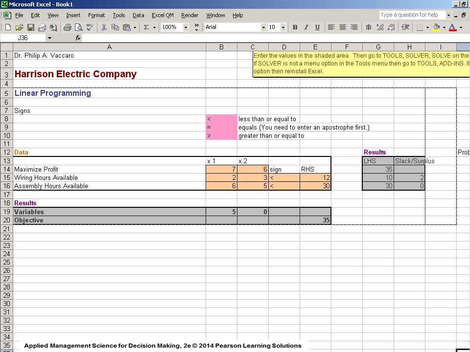
5. Harrison Electric Company
PURE INTEGER PROBLEM
The Harrison Electric Company produces two products: old-fashioned
chandeliers and ceiling fans. Both products require a two-step process
involving wiring and assembly.
It takes 2 hours to wire each chandelier and 3 hours to wire a ceiling
fan.
Final assembly of the chandeliers and fans requires 6 and 5 hours, re-
spectively.
The production capability is such that only 12 hours of wiring time and
30 hours of assembly time are available.
If each chandelier produced nets the firm $7.00 and each fan $6.00, the
Production mix decision can be formulated using LP as follows:

6. Harrison Electric Company
Maximize profit = $7.00 X1 + $6.00 X2
subject to:
2X1 + 3X2 =< 12 ( wiring hours )
6X1 + 5X2 =< 30 ( assembly hours )
X1, X2 => 0
where:
X1 = number of chandeliers produced
X2 = number of ceiling fans produced
The Model

7. Harrison Electric CompanyX2
+ = Possible Integer Solution 6 5 4 3 2 1
6X1 + 5X2 =< 30 ( assembly hours )
Optimal LP Solution
( X1 = 3.75 , X2 = 1.5 , Profit = $35.25 ) + + + +
2X1 + 3X2 =< 12 ( wiring hours ) + + + + X1

8. Harrison Electric Company
The optimal solution is X1 = 3.75 chandeliers and X2 = 1.5 ceiling
fans.
Rounding to X1 = 4 and X2 = 2 makes the solution unfeasible.
Rounding to X1 = 4 and X2 = 2 is probably not the optimal
feasible integer solution either .
There are 18 feasible integer solutions to this problem.
The optimal integer solution is X1 = 5 and X2 = 0 , with a total
profit of $
The integer restriction reduced profit from $35.25 to $35.00
An integer solution can never produce a greater profit than the
LP solution to the same problem.
DISCUSSION

9. Harrison Electric Company
Listing all feasible solutions and selecting the one with the best objective
function value is called the enumeration method. This can be virtually
impossible for large problems where the number of feasible solutions is
extremely large !
Chandeliers ( X1 )
Ceiling Fans ( X2 )
Profit ( Z )
$0.00 1 7 2 14 3 21 4 28 5 35 6 13 20
Integer
optimal
solution

10. Harrison Electric Company
Listing all feasible solutions and selecting the one with the best objective
function value is called the enumeration method. This can be virtually
impossible for large problems where the number of feasible solutions is
extremely large !
Chandeliers ( X1 )
Ceiling Fans ( X2 )
Profit ( Z ) 3 1 27 4 34 2 12 19 26 33 18 25 24
Rounding
optimal
solution

11. Branch-and-Bound Method
Solve the original problem using linear programming.
If the answer satisfies the integer constraints, we are
done.
If not, this value provides an initial upper bound for
the objective function.
Find any feasible solution that meets the integer con-
straints for use as a lower bound. Usually, rounding
down each variable will accomplish this.

12. Branch-and-Bound Method
Branch on one variable from step 1 that does not
have an integer value. Split the problem into two
subproblems based on integer values that are above
and below the noninteger value.
For example, if X2 = 3.75 was in the optimal linear
programming solution, introduce constraint X2 => 4
in the first subproblem, and X2 =< 3 in the second
subproblem.

13. Branch-and-Bound Method
Create nodes at the top of these new branches by
solving the new problems.

14. Branch-and-Bound Method
5. a If a branch yields a solution that is not feasible,
terminate the branch.
5. b If a branch yields a solution that is feasible, but
not an integer solution, go to step 6.
5. c If the branch yields a feasible integer solution,
look at the objective function. If its value equals
the upper bound, an optimal solution has been
reached.
If it is not equal to the upper bound, but exceeds
the lower bound, set it as the new lower bound
and go to step 6.
Finally, if it is less than the lower bound, terminate
this branch.

15. Branch-and-Bound Method
Examine both branches again and set the
upper bound equal to the maximum value
of the objective function at all final nodes.
If the upper bound equals the lower bound,
stop.
If not, go back to step 3 .

16. Harrison Electric Company
REVISITED
Harrison Electric Company
Maximize profit = $7.00 X1 + $6.00 X2
subject to:
2X1 + 3X2 =< 12 ( wiring hours )
6X1 + 5X2 =< 30 ( assembly hours )
X1, X2 => 0
where:
X1 = number of chandeliers produced
X2 = number of ceiling fans produced
The Model

17. Harrison Electric Company
REVISITED
Harrison Electric Company X2
+ = Possible Integer Solution 6 5 4 3 2 1
6X1 + 5X2 =< 30 ( assembly hours )
Optimal NON-INTEGER LP Solution
( X1 = 3.75 , X2 = 1.5 , Profit = $35.25 ) + + + +
2X1 + 3X2 =< 12 ( wiring hours ) + + + + X1

18. Branch-and-Bound Method
Since X1 and X2 are not integers, the solution is not valid.
The profit of $35.25 will be the initial upper bound.
Rounding down gives X1 = 3, X2 = 1, profit = $27.00 , which
is feasible and can be used as a lower bound.
X1=3.75
X2=1.5
P=35.25
Upper Bound = $35.25
Lower Bound = $27.00
(rounding down)
Original
Non-Integer
Solution

19. Branch-and-Bound Method
We divide the problem into two subproblems, A and B
We can branch on either the non-integer X1 or X2
We choose X1 this time
X1=3.75
X2=1.5
P=35.25
Upper Bound = $35.25
Lower Bound = $27.00
(rounding down)
Original
Non-Integer
Solution

20. Branch-and-Bound Method
Subproblem A
Max Z = $7X1 + $6X2
s.t X1 + 3X2 =< 12
6X1 + 5X2 =< 30
X1 => 4
Subproblem B
Max Z = $7X1 + $6X2
s.t X1 + 3X2 =< 12
6X1 + 5X2 =< 30
X1 =< 3
X1=3.75
X2=1.5
P=35.25
Upper Bound = $35.25
Lower Bound = $27.00
(rounding down)
Original
Non-Integer
Solution

21. Branch-and-Bound Method
Subproblem A
Noninteger Solution
Upper Bound = $35.20
Lower Bound = $33.00
X1=4
X2=1.2
P=35.20
X1=3.75
X2=1.5
P=35.25
Upper Bound = $35.25
Lower Bound = $27.00
(rounding down)
Subproblem B
X1=3
X2=2
P=33.00
This Branch
Solution Is Integer
New Lower Bound $33.00

22. Branch-and-Bound Method
Subproblem A is now branched into two new
subproblems, C and D
Subproblem C has the additional constraint of
X2 => 2
Subproblem D has the additional constraint of
X2 =< 1
The logic here is that since A’s optimal solution
of X1 = 1.2 is not feasible, the integer feasible
answer must lie at X2 => 2 or X2 =< 1

23. Branch-and-Bound Method
Subproblem C
Max Z = $7X1 + $6X2
s.t X1 + 3X2 =< 12
6X1 + 5X2 =< 30
X1 => 4
X2 => 2
Subproblem D
Max Z = $7X1 + $6X2
s.t X1 + 3X2 =< 12
6X1 + 5X2 =< 30
X1 => 4
X2 =< 1
Subproblem C has no feasible solution whatsoever because the first
two constraints are violated if X1 => 4 and X2 => 2 constraints are
observed. We terminate this branch and do not consider its solution.
Subproblem D’s solution is X1 = 4.17, X2 = 1, profit = $ This non-
integer solution yields a new upper bound of $35.16.

24. Branch-and-Bound Method
Subproblem C No
Feasible
Solution
Subproblem A
X2 => 2
X1=4
X2=1.2
P=35.20
X1 => 4
X1=3.75
X2=1.5
P=35.25
Subproblem D
X2 =< 1
X1=4.17
X2=1
P=35.16
Subproblem B
X1 =< 3
X1=3
X2=2
P=33.00
Upper Bound
= $35.16
Lower Bound
= $33.00

25. Branch-and-Bound Method
Finally, we create subproblems E and F and solve for X1 and X2 with
the additional constraints X1 =< 4 and X1 => 5 .
Subproblem E
Max Z = $7X1 + $6X2
s.t X1 + 3X2 =< 12
6X1 + 5X2 =< 30
X1 => 4
X1 =< 4
X2 =< 1
Subproblem F
Max Z = $7X1 + $6X2
s.t X1 + 3X2 =< 12
6X1 + 5X2 =< 30
X1 => 4
X1 => 5
X2 =< 1

26. Full Branch-and-Bound Solution
Harrison Electric Company
Full Branch-and-Bound Solution
Subproblem C
Subproblem A No
Feasible
Solution
X2 => 2
X1=4
X2=1.2
P=35.20
Subproblem E
X1=4
X2=1
P=34.00
X1 => 4
Feasible
Integer
Solution
X1=3.75
X2=1.5
P=35.25
X2 =< 1
Subproblem D
X1 =< 4
X1=4.17
X2=1
P=35.16
Subproblem B
Subproblem F
X1 =< 3
X1=3
X2=2
P=33.00
X1=5
X2=0
P=35.00
Feasible
Integer
Optimal
Solution
X1 => 5
The stopping rule for the branching process is that we continue until the new upper
bound is less than or equal to the lower bound or no further branching is possible.
The latter is the case here since both branches yielded feasible integer solutions.

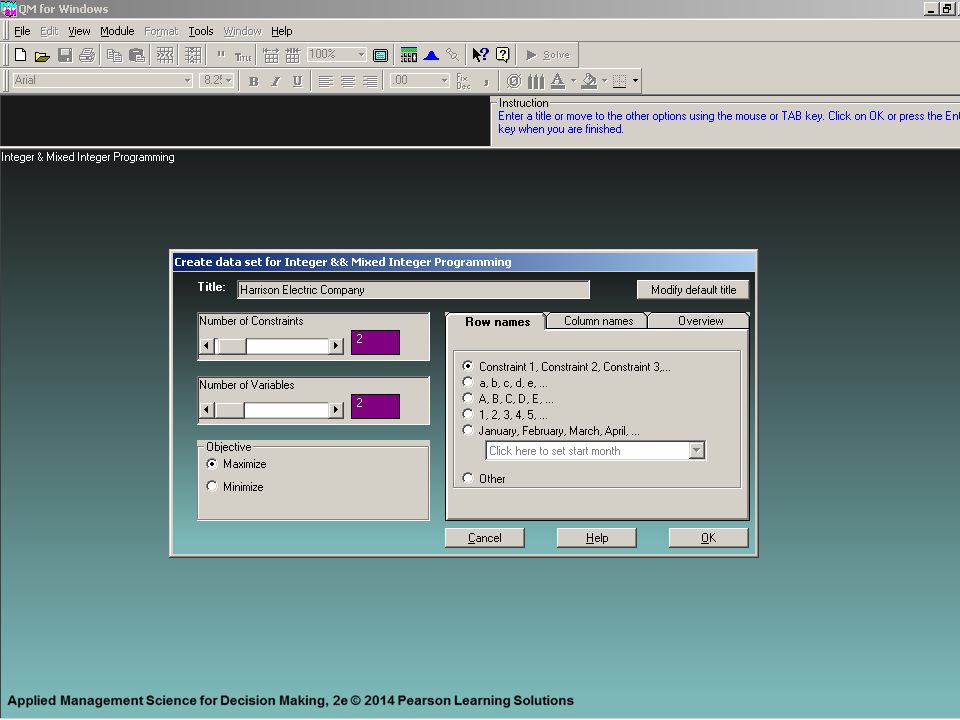
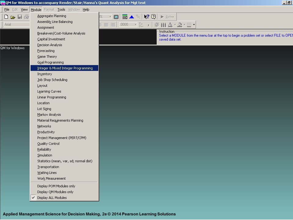
27. Integer Programming with QM for WINDOWS Harrison Electric Company

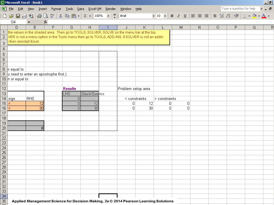
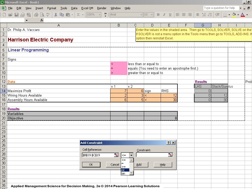
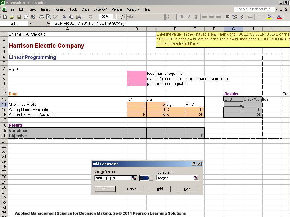
38. Integer Programming Using
The
Harrison
Electric
Company

53. Mixed Integer Programming
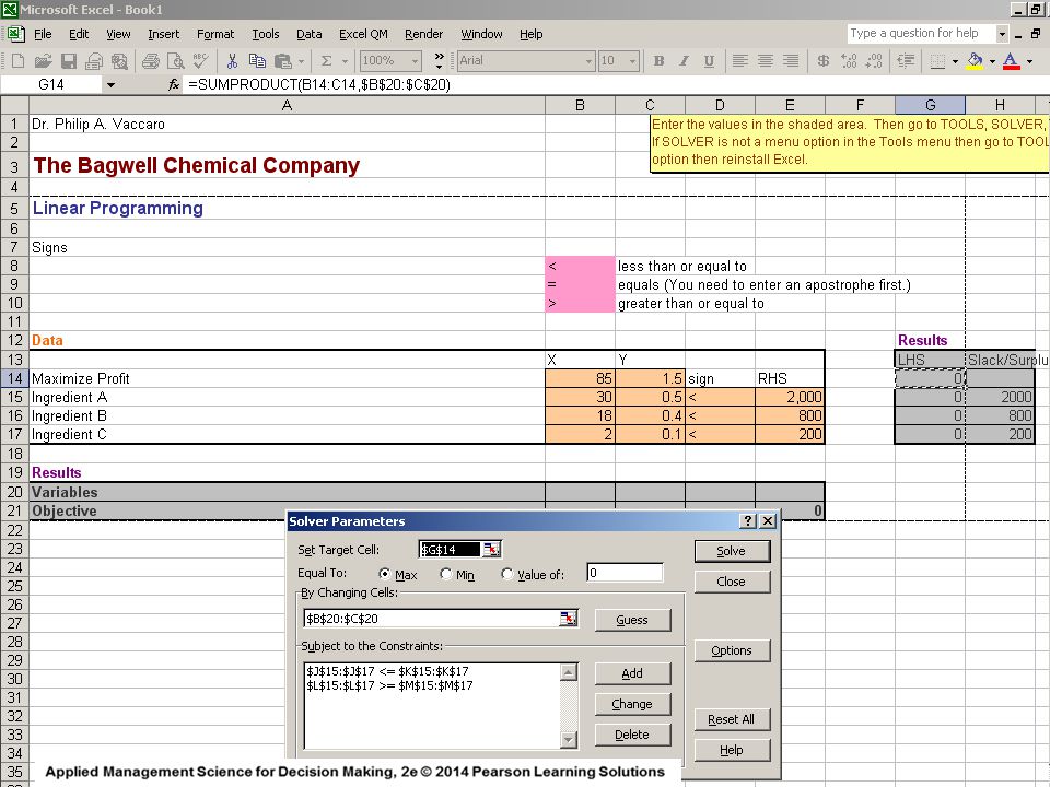
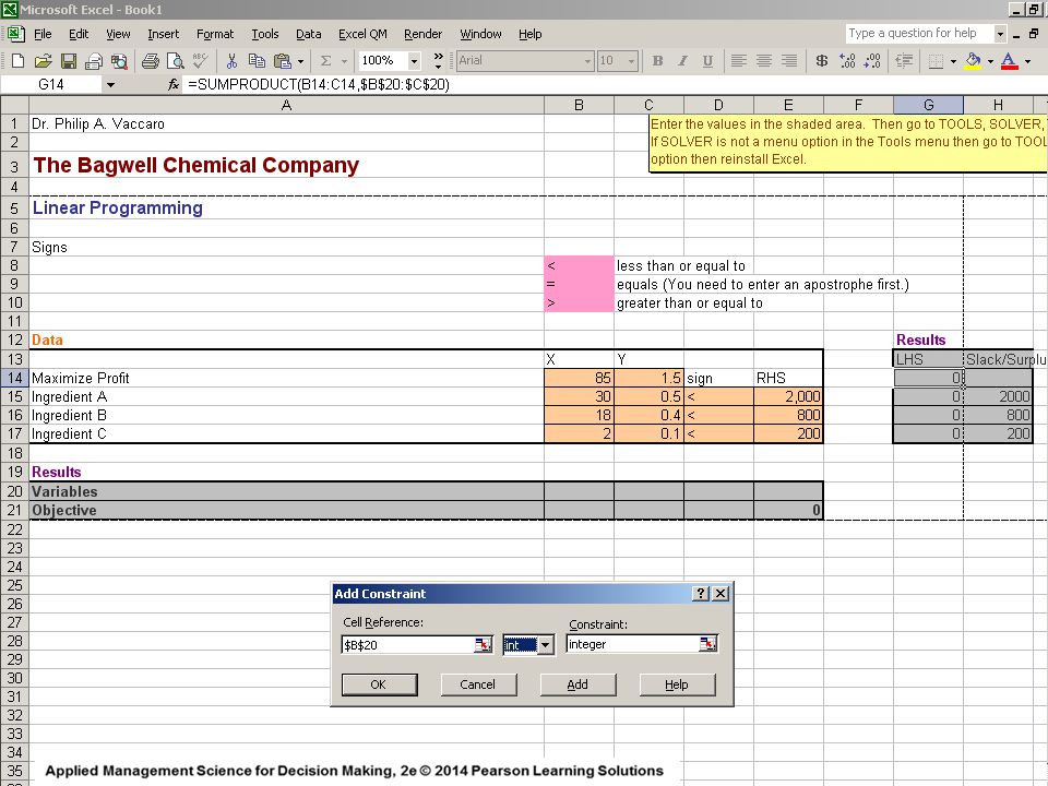
The Bagwell Chemical Company produces two industrial
chemicals.
The first product, xyline, must be produced in 50-pound
bags.
The second, hexall, is sold by the pound in dry bulk and
hence can be produced in any quantity.
Both xyline and hexall are composed of three ingredients:
A, B, and C as follows:

54. The Bagwell Chemical Co.
Amount per
50-Pound Bag
of Xyline (lb)
Pound
of Hexall (lb)
Amount of
Ingredients
Available 30
0.5
2,000 lb - A 18
0.4
800 lb - B 2
0.1
200 lb - C
Bagwell sells 50-pound bags of xyline for $85.00 and hexall in any weight for $1.50 per pound.
By formulating the usage coefficients for each 50-pound bag of Xyline, rather than for each
pound of Xyline, the program will automatically compute the purchase quantity for Xyline in
50-pound bag units, if an integer output is required.

55. The Bagwell Chemical Co.
Maximize Z = $85.00 X + $1.50 Y
s.t.
30 X Y <= 2,000
18 X Y <=
2 X Y <=
X,Y => 0 and X integer
The Model
X = number of 50-pound bags of xyline produced ; Y = number of pounds of hexall (in dry bulk) mixed

56. The Bagwell Chemical Co.
The Solution
The Integer Solution The Optimal Solution
X = 44 bags of xyline
Y = 20 pounds of hexall
Z = $3,770.00
X = bags of xyline
Y = 0 pounds of hexall
Z = $3,777.78

57. Integer Programming with QM for WINDOWS Bagwell Chemical Company
Mixed Integer Program
for
Bagwell Chemical Company

67. Mixed Integer Programming Using
The
Bagwell
Chemical
Company

80. Modeling with Binary Variables
Typically, a ‘0-1’ variable is assigned a value of 0
if a certain condition is not met, and a value of ‘1’
if the condition is met.
Another name for a ‘0-1’ variable is a binary vari-
able.
A common problem of this type is the assignment
problem which involves deciding which individuals
are assigned to a set of jobs. A value of 1 indicates
a person is assigned to a specific job. A value of 0
indicates the assignment was not made.

81. Capital Budgeting Example
A common capital budgeting decision involves
selecting from a set of possible projects when
budget limitations make it impossible to select
all of these.
A separate ‘0-1’ variable can be defined for each
project.

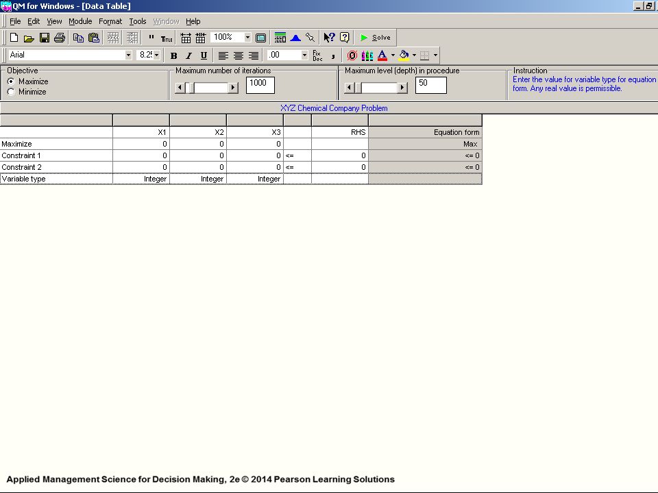
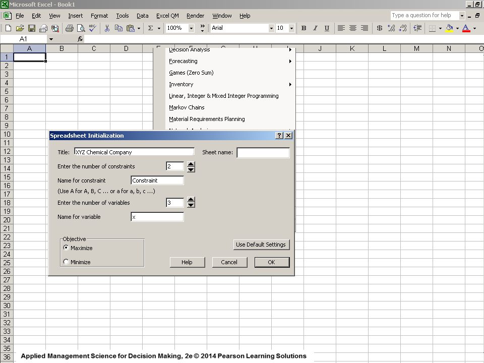
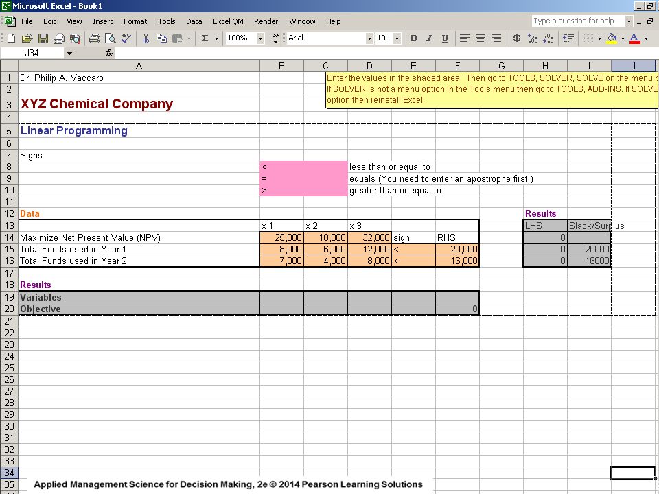
82. XYZ Chemical Company
XYZ is considering three possible improvement projects
for its plant: a new catalytic converter, a new software
program for controlling operations, and expanding the
warehouse used for storage.
Capital requirements and budget limitations in the next
two years prevent the firm from underatking all of these
at this time.
The net present value of each of the projects , the capital
requirements, and the available funds for the next two
years are given on the next slide.
NPV is the
future value
of a project
discounted
back to the
present time

83. XYZ Chemical Company PROJECT Year 1 Year 2 $25,000. $8,000. $7,000.
Net
Present Value
Year 1
Capital Requirement
Year 2
Capital
Requirement
Catalytic Converter
$25,000.
$8,000.
$7,000.
Software
$18,000.
$6,000.
$4,000.
Warehouse Expansion
$32,000.
$12,000.
Budget Limitations
$20,000.
$16,000.
PROJECT

84. XYZ Chemical Company Maximize NPV of projects undertaken subject to:
Total funds used in year 1 =< $20,000.
Total funds used in year 2 =< $16,000.
We define the decision variables as:
X1 = if catalytic converter project is funded
0 otherwise
X2 = if software project is funded
X3 = 1 if warehouse expansion project is funded

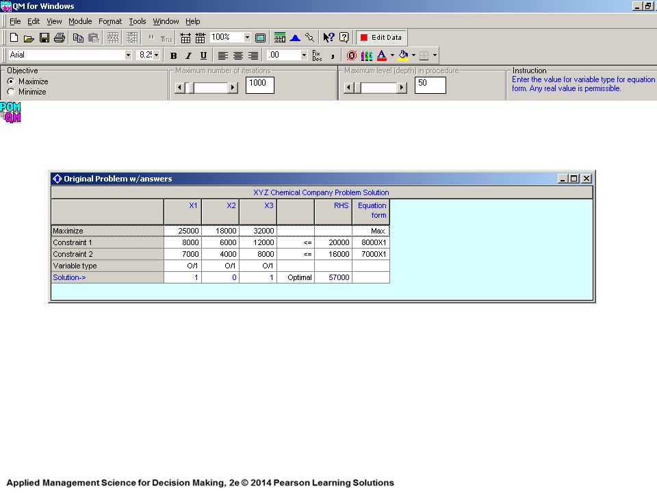
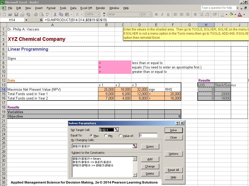
85. XYZ Chemical Company Maximize NPV = 25,000 X1 + 18,000 X2 + 32,000 X3
subject to:
8,000 X1 + 6,000 X2 + 12,000 X3 =< 20,000
7,000 X1 + 4,000 X2 + 8,000 X3 =< 16,000
X1, X2, X3 = 0 or 1
The Model

86. XYZ Chemical Company and the warehouse expansion project, but not the
The Solution
X1 = 1 , X2 = 0 , X3 = 1 , Z = 57,000
The firm should fund the catalytic converter project,
and the warehouse expansion project, but not the
new software project.
The net present value of these investments will be
$57,000.00

87. Integer Programming with QM for WINDOWS Binary Variable Modeling
for the
XYZ Chemical Company

97. XYZ
Chemical
Company

110. XYZ Chemical Company Limiting the Number of Alternatives Selected
Suppose that XYZ Chemical Company is required to select no
more than two of the three projects regardless of the funds
available.
This could be modeled by adding the following constraint to
the problem:
X1 + X2 + X3 =< 2
If we wished to force the selection of exactly two of the three
projects for funding, the following constraint should be used:
X1 + X2 + X3 = 2
This forces exactly two of the variables to have values of 1,
whereas the other variable must have a value of 0.

111. XYZ Chemical Company Dependent Selections
At times the selection of one project depends in some way
upon the selection of another project. This situation can be
modeled with the use of 0-1 variables.
Suppose that the new catalytic converter could be purchased
only if the software was purchased also. The following con-
straint would force this to occur:
X1 <= X2 or X1 - X2 <= 0
Thus, if the software is not purchased, the value of X2 is 0, and
the value of X1 must be 0 also because of this constraint.
However, if the software is purchased ( X2 = 1 ), then it is possi-
ble that the catalytic converter could be purchased ( X1 = 1)
also, although this is not required.

112. XYZ Chemical Company Dependent Selections
If we wished for the catalytic converter and the software
projects to either both be selected or both not be selected,
we should use the following constraint:
X1 = X2 or X1 - X2 = 0
Thus, if either of these variables is equal to 0, the other
must be 0 also.
If either of these variables is equal to 1, the other must
be 1 also.

113. Fixed-Charge Problem Often firms are faced with decisions involving
a fixed charge that will affect the cost of future
operations.
Building a new factory or entering into a long-
term lease on an existing facility would involve
a fixed cost that might vary depending upon the
size of the facility and the location.
Once a factory is built, the variable production
costs will be affected by the labor cost in the
particular city where it is located.

114. Acme Manufacturing, Inc.
FIXED-CHARGE PROBLEM EXAMPLE
Acme Manufacturing is planning to build at least one
new plant, and three cities are being considered:
Baytown, TX; Lake Charles, LA; and Mobile, AL.
Once the plant or plants have been constructed, the
firm wishes to have sufficient capacity to produce at
least 38,000 units each year.
The costs associated with the possible locations are
shown on the following slide.

115. Acme Manufacturing, Inc.
SITE
ANNUAL
FIXED COST
VARIABLE COST PER UNIT
ANNUAL CAPACITY
Baytown
$340,000.
$32.
21,000
Lake Charles
$270,000.
$33.
20,000
Mobile
$290,000.
$30.
19,000

116. Acme Manufacturing, Inc.
The objective function is to minimize the total of
the fixed cost and the variable cost.
Total production capacity is at least 38,000 units.
The number of units produced at Baytown is ‘0’
if the plant is not built, and no more than 21,000
if the plant is built.
The number of units produced at Lake Charles is
‘0’ if the plant is not built, and no more than 20,000
The number of units produced at Mobile is ‘0’ if
the plant is not built, and no more than 19,000 if
the plant is built.

117. Acme Manufacturing, Inc.
The decision variables:
X1 = ‘1’ if the factory is built in Baytown ; ‘0’ otherwise.
X2 = ‘1’ if the factory is built in Lake Charles ; ‘0’ otherwise.
X3 = ‘1’ if the factory is built in Mobile ; ‘0’ otherwise.
X4 = number of units produced at Baytown plant.
X5 = number of units produced at Lake Charles plant.
X6 = number of units produced at Mobile plant.

118. Acme Manufacturing, Inc.
Texas
Louisiana
Minimize Cost = 340,000 X1 + $270,000 X2 + $290,000 X3
X X X6
subject to:
X4 + X5 + X6 => 38,000
X4 =< 21,000 X1
X5 =< 20,000 X2
X6 =< 19,000 X3
X1, X2, X3 = 0 or 1 ; X4, X5, X6 => 0 and integer
The Model

119. Acme Manufacturing, Inc.
Proposed Site
If X1 = 0 , meaning Baytown plant is not built, then
X4 , number of units produced at Baytown plant,
must equal 0 also, due to the second constraint.
If X1 = 1 , then X4 may be any integer value less
than or equal to the limit of 21,000 units.
The third and fourth constraints are similarly used
to guarantee that no units are produced at the
other locations if the plants are not built.

120. Acme Manufacturing, Inc.
X1 = 0
X2 = 1
X3 = 1
X4 = 0
X5 = 19,000
X6 = 19,000
Z = 1,757,000.00
Optimal Solution
Factories will be built at
Lake Charles and Mobile.
Each of these wil produce
19,000 units each year.
Total annual cost will be
$1,757,000.00

121. Financial Investment Example
Numerous financial applications exist with
binary variables.
A very common type of problem involves
selecting from a group of investment op-
portunities.

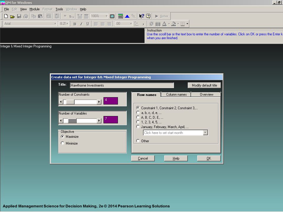
122. Hawthorne Investments
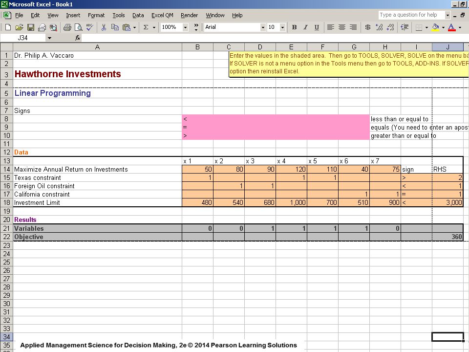
Hawthorne Investments specializes in recommending oil
stock portfolios for wealthy clients. One such client has
made the following specifications:
At least two Texas oil firms must be in the portfolio.
No more than one investment can be made in foreign
oil companies.
One of the two California oil stocks must be purchased.
The client has up to $3 million available for investments
and insists on purchasing large blocks of shares of each
company he invests in.
The objective is to maximize annual return on investment
subject to the constraints.

123. Hawthorne Investments
Stocks Being Considered
Hawthorne Investments
The firm is being forced by the client
to buy shares in “blocks” so the
cost per “block” is shown below.
Stock
Company
Name
Expected
Annual Return
($1,000s)
Cost for Block
Of Shares 1
Trans-Texas Oil 50
480 2
British Petroleum 80
540 3
Dutch Shell 90
680 4
Houston Drilling
120
1,000 5
Texas Petroleum
110
700 6
San Diego Oil 40
510 7
California Petro 75
900

124. Hawthorne Investments
To formulate this as a 0-1 integer programming
problem, let Xi be a ‘0-1’ integer variable, where
Xi = 1 if the stock is purchased and Xi = 0 if the
stock is not purchased.

125. Hawthorne Investments
Maximize return = 50 X X X X4
+ 110 X X X7
subject to:
X1 + X4 + X5 => 2 ( Texas constraint )
X2 + X3 =< 1 ( foreign oil constraint )
X6 + X7 = 1 ( California constraint )
480 X X X3 + 1,000 X4
+ 700 X X X7 =< 3,000 ( $3 million limit )
All variables must be 0 or 1 in value.
The Model

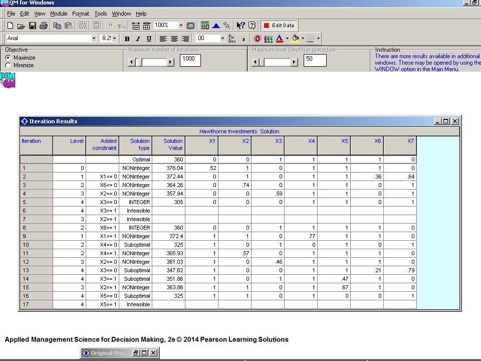
126. Hawthorne Investments
The Optimal Solution
Hawthorne should invest in
Dutch Shell
Houston Drilling
Texas Petroleum
San Diego Oil
and not in
Trans-Texas Oil
British Petroleum
California Petro
The expected return is
$360,000.00
X3 = 1
X4 = 1
X5 = 1
X6 = 1
X1 = 0
X2 = 0
X7 = 0
Z = 360,000

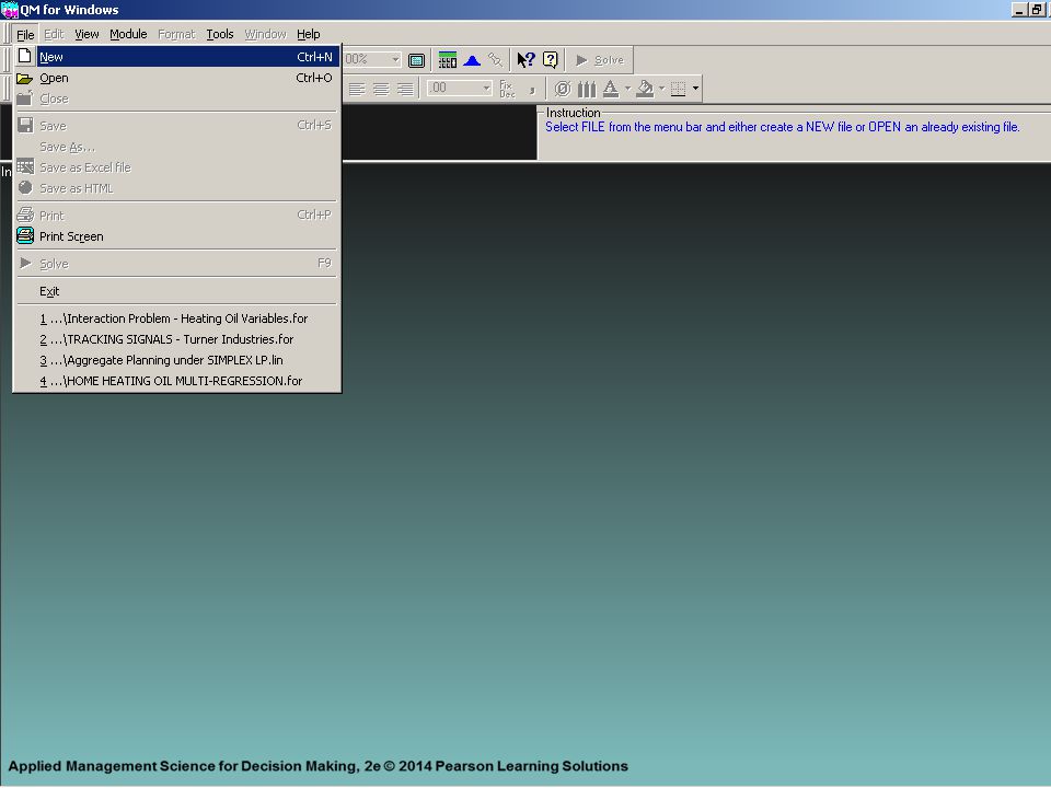
127. 0-1 Integer Programming Using
Hawthorne
Investments
Problem

141. 0-1 Integer Programming with QM for WINDOWS Hawthorne Investments
Problem

148. Applied Management Science for Decision Making, 2e © 2014 Pearson Learning Solutions