Download presentation
Presentation is loading. Please wait.

1
Multiclass SVM and Applications in Object Classification
Yuval Kaminka, Einat Granot Advanced Topics in Computer Vision Seminar Faculty of Mathematics and Computer Science Weizmann Institute May 2007

2
Outline Motivation and Introduction Classification Algorithms
K-Nearest neighbors (KNN) SVM Multiclass SVM DAGSVM SVM-KNN Results - A taste of the distance Shape distance (shape context, tangent) Texture (texton histograms)
 SVM. Multiclass SVM. DAGSVM. SVM-KNN. Results - A taste of the distance. Shape distance (shape context, tangent) Texture (texton histograms)")
3
Object Classification
?

4
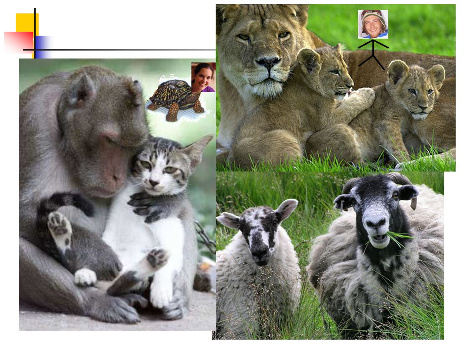
Motivation – Human Visual System
Large Number of Categories (~30,000) Discriminative Process Small Set of Examples Invariance to transformation Similarity to Prototype instead of Features
 Discriminative Process. Small Set of Examples. Invariance to transformation. Similarity to Prototype instead of Features.")
5
Similarity to Prototypes Vs Features
No need for Feature Space Easy to enlarge number of categories Includes spatial relation between features No need for feature definition, for example in the tangent distance

6
D( ) , Distance Function Similarity is defined by Distance Function
Easy to adjust to different types (Shape, Texture) Can include invariance to intra-class transformations
 Can include invariance to intra-class transformations.")
7
Distance Function – simple example
) = ) = || 2.1, 27, 31, 15, 8 . - || 13, 45, 22.5, 78, 91 ? , , 2.1 27 31 .
 = ) = || 2.1, 27, 31, 15, || 13, 45, 22.5, 78, 91. , ,")
8
Outline Motivation and Introduction Classification Algorithms
K-Nearest neighbors (KNN) SVM Multiclass SVM DAGSVM SVM-KNN Results - A taste of the distance Shape distance (shape context, tangent) Texture (texton histograms)
 SVM. Multiclass SVM. DAGSVM. SVM-KNN. Results - A taste of the distance. Shape distance (shape context, tangent) Texture (texton histograms)")
9
A Classic Classification Problem
Training Set S: (X1..Xn), with class label (Y1.. Yn) Given a query image q, determine its label X2 X3 X1 X5 q X4 X6 X7
, with class label (Y1.. Yn) Given a query image q, determine its label. X2. X3. X1. X5. q. X4. X6. X7.")
10
Nearest Neighbor (NN) ?
")
11
K-Nearest Neighbor (KNN)
? K = 3

12
K-NN Pros Simple, yet outperforms other methods Low Complexity: O(Dּn)
D - the cost per one distance function calculation No need for Feature Space definition No computational cost for adding new categories n ∞ ==> Error Rate Bayes optimal Bayes Optimal – A classifiers that always classify the classification that will get maximum probability, going over all possible hypothesis

13
K-NN Cons Complete Set Missing Set NN SVM
P. Vincent et al., K-local hyperplane and convex distance nearest neighbor algorithms, NIPS 2001

14
Outline Motivation and Introduction Classification Algorithms
K-Nearest neighbors (KNN) SVM Multiclass SVM DAGSVM SVM-KNN Results - A taste of the distance Shape distance (shape context, tangent) Texture (texton histograms)
 SVM. Multiclass SVM. DAGSVM. SVM-KNN. Results - A taste of the distance. Shape distance (shape context, tangent) Texture (texton histograms)")
15
SVM Two class classification algorithm
Hyperplane – תת-קבוצה של וקטורים במימד n-1 שמגדיר הפרדה במימד ה-n. Linear Hyperplane – Hyperplane שעובר דרך הראשית Class 1 We’re looking for a hyperplane that best separates the classes Some of the slides on SVM are adapted with permission from Martin Law’s presentation on SVM

16
As far away as possible from the data of both classes
SVM - Motivation Class 2 Class 2 Class 1 Class 1 As far away as possible from the data of both classes

17
SVM – A learning algorithm
KNN – simple classification, no training Class 1 Class 2 SVM – a learning algorithm Training – find the hyperplane Classification – label a new query Two Phases:

18
SVM – Training Phase We’re looking for (w,b) that will:
Class 2 ~b wTx+b=0 Class 1 We’re looking for (w,b) that will: Classify correctly the classes Give maximum margins
 that will: Classify correctly the classes. Give maximum margins.")
19
1. Correct classification
{x1, ..., xn} our training set wTx+b=0 Class 1 Correct classification: wTxi+b>0 for green, and wTxi+b<0 for red Assume the labels {y1.. yn} are from the set {-1,1}:

20
2. Margin maximization Class 2 m Class 1 m = ?

21
2. Margin maximization m We can scale (w,b) (w,b), >0
|wTz+b| ||w|| Class 2 z m Class 1 We can scale (w,b) (w,b), >0 Won’t change classification: wTx+b>0 wTx+b>0 Get a desired distance: |wTz+b|=a =1/a, |wTz+b|=1
 (w,b), >0. Won’t change classification: wTx+b>0 wTx+b>0. Get a desired distance: |wTz+b|=a =1/a, |wTz+b|=1.")
22
SVM as an Optimization Problem
Maximize margins Correct Classification Solve optimization problem with constraints We can find a1.. an, such that: Langrangian multipliers C.J.C. Burges. A Tutorial on Support Vector Machines for Pattern Recognition, 1998.

23
SVM as an Optimization Problem
Maximize margins Correct Classification Classic optimization problem with constraints לשנות x ל-w ולתקן למטה ל-xi s.t.

24
SVM as an Optimization Problem
s.t. There must exist positive a1.. an such that: And in our case: There must exist positive a1.. an such that: gi(x) f(x)
 f(x)")
25
Support Vectors xi with ai>0 are called support vectors (SV)
Class 2 a=0 a>0 a=0 a=0 a>0 a=0 a>0 a=0 a=0 Class 1 xi with ai>0 are called support vectors (SV) w is determined only by the SV
 w is determined only by the SV.")
26
Allowing errors We would now like to minimize wTx+b=1 wTx+b=0 wTx+b=-1
Class 2 wTx+b=1 Class 1 wTx+b=0 wTx+b=-1 We would now like to minimize

27
Allowing errors As before we get: Class 2 Class 1

28
SVM – Classification phase
q Class 1 Compute wTq+b Classify as class 1 if positive, and class 2 otherwise

29
Upgrade SVM We only need to calculate inner products
In order to find a1.. an we need to calculate xiTxj i,j In order to classify a query q we need to calculate:

30
Feature Expansion f(.) Extended space Input space f(.)
( 1 , x , y , xy , x2 , y2 ) (x , y) Problem: too expensive!
 (x , y) Problem: too expensive!")
31
Solution: The Kernel Trick
We only need to calculate inner products f( ) f(.) Find a kernel function K such that:
 f(.) Find a kernel function K such that:")
32
The Kernel Trick We only need to calculate inner products
In order to find a1.. an we need to calculate xiTxj i,j Build a kernel matrix MnXn: M[i,j]= (xi)T(xj)=K(xi,xj) In order to classify a query q we need to calculate wTq+b:
T(xj)=K(xi,xj) In order to classify a query q we need to calculate wTq+b:")
33
Inner product Distance Function
We only need to calculate inner products In our case: convert to distance function Parallelogram law: ||u+v||^2+||u-v||^2=2||u||^2+2||v||^2 From “origin” Pairwise distance

34
Inner product Distance Function
Use the fact that we only need to calculate inner products In order to find a1.. an we need to calculate xiTxj i,j Build a distance matrix DnXn: D[i,j] = xiTxj = 1/2ּ[d(xi,0)+d(xj,0)-d(xi,xj)] In order to classify a query q we need to calculate wTq+b:
+d(xj,0)-d(xi,xj)] In order to classify a query q we need to calculate wTq+b:")
35
SVM Pros and Cons Pros: Easy to integrate different distance functions
Fast classification of new objects (depends on SV) Good performance even with small set of examples Cons: Slow training ( O(n2), n=# of vectors in training set ) Separates only 2 classes להזכיר שהחיסרון הראשון "נעלם" כאשר מדובר על סט קטן של דוגמאות
 Good performance even with small set of examples. Cons: Slow training ( O(n2), n=# of vectors in training set ) Separates only 2 classes. להזכיר שהחיסרון הראשון נעלם כאשר מדובר על סט קטן של דוגמאות.")
36
Outline Motivation and Introduction Classification Algorithms
K-Nearest neighbors (KNN) SVM Multiclass SVM DAGSVM SVM-KNN Results - A taste of the distance Shape distance (shape context, tangent) Texture (texton histograms)
 SVM. Multiclass SVM. DAGSVM. SVM-KNN. Results - A taste of the distance. Shape distance (shape context, tangent) Texture (texton histograms)")
37
Multiclass SVM Extend SVM for multi-classes separation
Nc = number of classes Class 2 Class 1 Class 5 Class 4 Class 3

38
Two approaches Class 1 Class 2 Class 3 Class 4
1-vs-rest 1-vs-1 DAGSVM Combine multi-binary-classifiers Generate one function based on single optimization problem

39
1-vs-rest Class 2 Class 1 Class 4 Class 3

40
1-vs-rest w2 w1 Class 2 Class 1 w3 w4 Nc classifiers Class 3 Class 4

41
1-vs-rest Class 2 Class 1 Class 3 Class 4 w2 w1 w3 w4
~ Similarity(q,SV3) q ~ Similarity(q,SV2) w1Tq+b1 ~ Similarity(q,SV1) ~ Similarity(q,SV4) Class 3 Class 4
 q. ~ Similarity(q,SV2) w1Tq+b1 ~ Similarity(q,SV1) ~ Similarity(q,SV4) Class 3. Class 4.")
42
argmax1≤i ≤Nc{Sim(q,SVi)}
1-vs-rest w2 w1 Class 2 Class 1 w3 w4 q Label(q)= argmax1≤i ≤Nc{Sim(q,SVi)} Class 3 Class 4
= argmax1≤i ≤Nc{Sim(q,SVi)} Class 3. Class 4.")
43
1-vs-rest After training we’ll have Nc decision functions:
fi(x)=wiTx+bi Class of query object q is determined by: argmax1≤i ≤Nc{ wiTx+bi } Pros: Only Nc classifiers to be trained and tested Cons: Every classifier use all vectors for training No bound on generalization error
=wiTx+bi. Class of query object q is determined by: argmax1≤i ≤Nc{ wiTx+bi } Pros: Only Nc classifiers to be trained and tested. Cons: Every classifier use all vectors for training. No bound on generalization error.")
44
1-vs-rest Complexity For training:
Nc classifiers, each using n vectors for finding hyperplane For classifying new objects: Nc classifiers, each is tested once, M=max number of SV

45
1-vs-1 Class 2 Class 1 Class 4 Class 3

46
1-vs-1 Nc(Nc-1)/2 classifiers Class 2 Class 1 Class 4 Class 3 W1,2
/2 classifiers Class 2 Class 1 Class 4 Class 3 W1,2")
47
1-vs-1 with Max Wins ☺ ☺ ☺ ☺ ☺ ☺ Class 2 Class 1 Class 4 Class 3 W1,2
q W2,3 ~ 2 or 4 ? Sign(w1,2Tq+b1,2) ~ 1 or 2 ? W1,3 ~ 1 or 3 ? W2,4 ~ 1 or 4 ? ~ 3 or 4 ? W3,4 ~ 2 or 3 ? Class 4 Class 3 ☺ ☺
 ~ 1 or 2 W1,3. ~ 1 or 3 W2,4. ~ 1 or 4 ~ 3 or 4 W3,4. ~ 2 or 3 Class 4. Class 3. ☺ ☺")
48
1-vs-1 with Max Wins ☺ ☺ ☺ ☺ ☺ ☺ Class 2 Class 1 Class 4 Class 3 W1,2
q W2,3 W1,3 W2,4 W3,4 Class 4 Class 3 ☺ ☺

49
1-vs-1 with Max Wins After training we’ll have Nc(Nc-1)/2 decision functions: fij(x)=sign(wijTx+bij) Class of query object x is determined by max-votes Pros: Every classifier use a small set of vectors for training Cons: Nc(Nc-1)/2 classifiers to be trained and tested No bound on generalization error
/2 classifiers to be trained and tested. No bound on generalization error.")
50
1-vs-1 Complexity For training:
Assume that every class contains ~ n/Nc instances Nc(Nc-1)/2 classifiers, each using ~2n/Nc vectors: For classifying new objects: Nc(Nc-1)/2 classifiers, each is tested once, M as before
/2 classifiers, each using ~2n/Nc vectors: For classifying new objects: Nc(Nc-1)/2 classifiers, each is tested once, M as before.")
51
What did we have so far? 1-vs-1 1-vs-rest Nc(Nc-1)/2 Nc
Class 1 Class 2 Class 3 Class 4 Class 1 Class 2 Class 3 Class 4 1-vs-1 1-vs-rest Nc(Nc-1)/2 Nc # of classifiers (each need to be trained and tested) ~2n/Nc n (all vectors) # of vectors for training (per classifier) No bound on generalization error להזכיר שכשהאימון נעשה על מס' דוגמאות קטן זה אמנם יתרון מבחינת סיבוכיות, אך יכול להיות חסרון מבחינת ביצועים
/2. Nc. # of classifiers (each need to be trained and tested) ~2n/Nc. n (all vectors) # of vectors for training (per classifier) No bound on generalization error. להזכיר שכשהאימון נעשה על מס דוגמאות קטן זה אמנם יתרון מבחינת סיבוכיות, אך יכול להיות חסרון מבחינת ביצועים.")
52
DAGSVM 1-vs-1 Decision DAG (DDAG) 4 1 2 3
3 4 2 3 4 1 2 1 2 3 2 3 not 1 not 2 not 3 not 4 4 1 2 3 Class 1 Class 2 Class 3 Class 4 W1,2 W1,3 W1,4 W2,3 W3,4 W2,4 J. C. Platt et al., Large margin DAGs for multiclass classification. NIPS, 1999.

53
Binary decision function Nc(Nc-1)/2 internal nodes
DDAG on Nc Classes Single root node 1 vs 4 3 vs 4 2 vs 4 1 vs 3 2 vs 3 1 vs 2 3 4 2 3 4 1 2 1 2 3 2 3 not 1 not 2 not 3 not 4 4 1 2 3 In every node: Binary decision function Nc(Nc-1)/2 internal nodes DAG Nc leaves, one per class
/2 internal nodes. DAG. Nc leaves, one per class.")
54
Building the DDAG 1 2 3 4 change list order no affect on results 4 3 2
1 vs 4 change list order no affect on results not 1 not 4 2 3 4 2 vs 4 1 2 3 1 vs 3 not 2 not 4 not 1 not 3 2 3 3 vs 4 2 vs 3 1 vs 2 3 4 1 2 4 3 2 1

55
Classification using DDAG
1 vs 4 W1,2 ~ 1 or 2 ? q Class 2 Class 1 ~ 1 or 4 ? not 1 not 4 W1,4 ~ 1 or 3 ? 2 3 4 2 vs 4 1 2 3 1 vs 3 W1,3 W2,3 W2,4 W3,4 not 2 not 4 not 1 not 3 בהנחה שה-classes ניתנים להפרדה והשוליים שמתקבלים אכן גדולים אזי הגיוני "להיפטר" מה-class שלא בחרנו לסווג אליה בכל פעם. 3 4 2 3 3 vs 4 2 vs 3 1 vs 2 1 2 Class 4 Class 3 4 3 2 1

56
DAGSVM Pros: Only Nc-1 classifiers to be tested
Every classifier uses a small set of vectors for training Bound on generalization error (~margins size) Cons: Less vectors for training worse classifier? Nc(Nc-1)/2 classifiers to be trained
 Cons: Less vectors for training worse classifier Nc(Nc-1)/2 classifiers to be trained.")
57
DAGSVM Complexity For training:
Assume that every class contains ~n/Nc instances Nc(Nc-1)/2 classifiers, each using ~2n/Nc vectors: For classifying new objects: Nc-1 classifiers, each is tested once M = max number of SV
/2 classifiers, each using ~2n/Nc vectors: For classifying new objects: Nc-1 classifiers, each is tested once. M = max number of SV.")
58
Classification complexity
Multiclass SVM DAGSVM 1-vs-1 1-vs-rest Nc # of classifiers O(Dּn2) O(DּNcn2) Training complexity O(M2ּNc) O(M2ּNc2) O(M1ּNc) Classification complexity
 O(DּNcn2) Training complexity. O(M2ּNc) O(M2ּNc2) O(M1ּNc) Classification complexity.")
59
Multiclass SVM comparison
Classification Training

60
Multiclass SVM - Summary
Training: Classification: Error rates: Bound of generalization error - only on DAGSVM In practice – 1-vs-1 and DAGSVM The “one big optimization” methods Similar error rates Very slow training – limited to small data sets 1-vs-rest DAGSVM / 1-vs-1 O(DּNcּn2) O(Dּn2) 1-vs-1 DAGSVM / 1-vs-rest O(DּMּNc2) O(DּMּNc)
 O(Dּn2) 1-vs-1. DAGSVM / 1-vs-rest. O(DּMּNc2) O(DּMּNc)")
61
So what do we have? Nearest Neighbor (KNN) SVM Fast
Suitable for multi-class Easy to integrate different distance functions Problematic with few samples SVM Good performance even with small set of examples No natural extension to multi-class Slow to train Class 1 Class 2

62
SVM KNN - From coarse to fine
Suggestion Hybrid system KNN SVM Zhang et al, SVM-KNN: Discriminative Nearest Neighbor Classification for Visual Category Recognition, 2006

63
Outline Motivation and Introduction Classification Algorithms
K-Nearest neighbors (KNN) SVM Multiclass SVM DAGSVM SVM-KNN Results - A taste of the distance Shape distance (shape context, tangent) Texture (texton histograms)
 SVM. Multiclass SVM. DAGSVM. SVM-KNN. Results - A taste of the distance. Shape distance (shape context, tangent) Texture (texton histograms)")
64
SVM KNN – General Algorithm
Calculate distance from query to training images Query image Class 1 Class 2 Class 3 Training images and query

65
SVM KNN – General Algorithm
Calculate distance from query to training images Pick K nearest neighbors Query image Class 1 Class 2 Class 3 Training images and query

66
SVM KNN – General Algorithm
Calculate distance from query to training images Pick K nearest neighbors Run SVM Query image Class 1 Class 2 Class 3 SVM works well with few samples Training images and query

67
SVM KNN – General Algorithm
Calculate distance from query to training images Pick K nearest neighbors Run SVM Label ! Query image Class 1 Class 2 Class 3 Query image Class 2 Training images and query

68
Training + Classification
Calculate distance from query to training images Pick K nearest neighbors Run SVM Label ! KNN SVM Classic process: Training Classification SVM-KNN Coarse Classification Final classification

69
Details Details Details
Calculate distance from query to training images Pick K nearest neighbors Run SVM Label ! KNN SVM Calculating distance is a heavy task Compute crude distance – faster Finding Kpotential images Ignore all other images Compute accurate distance Only relative to the Kpotential images L2 Accurate Kpotential

70
Details Details Details
Calculate distance from query to training images Pick K nearest neighbors Run SVM Label ! KNN SVM Complexity: Crude distance Accurate distance L2 Accurate Kpotential

71
Details Details Details
Calculate distance from query to training images Pick K nearest neighbors Run SVM Label ! KNN SVM If K neighbors are from the same class Done

72
Details Details Details
Calculate distance from query to training images Pick K nearest neighbors Run SVM Label ! KNN SVM Construct pairwise inner product matrix Improvement – cache distance calculation

73
Details Details Details
Calculate distance from query to training images Pick K nearest neighbors Run SVM Label ! KNN SVM Selected SVM: DAGSVM (faster) Complexity: 1 vs 4 3 vs 4 2 vs 4 1 vs 3 2 vs 3 1 vs 2
 Complexity: 1 vs 4. 3 vs 4. 2 vs 4. 1 vs 3. 2 vs 3. 1 vs 2.")
74
Complexity Total complexity DAGSVM training complexity
Calculate distance from query to training images Pick K nearest neighbors Run SVM Label ! KNN SVM Total complexity DAGSVM training complexity

75
SVM KNN – continuum Defining an SVM-KNN continuum: NN SVM
K = n (#images) NN KNN SVM SVM More than MAJ Biological motivation Human visual system
 NN. KNN. SVM. SVM. More than MAJ. Biological motivation Human visual system.")
78
SVM KNN Summary Similarity to prototypes
Combining Advantages from both methods NN – Fast, suitable for multiclass SVM – performs well with few samples and classes Compatible with many types of distance functions Biological motivation: Human visual system Discriminative process

79
Outline Motivation and Introduction Classification Algorithms
K-Nearest neighbors (KNN) SVM Multiclass SVM DAGSVM SVM-KNN Results - A taste of the distance Shape distance (shape context, tangent) Texture (texton histograms)
 SVM. Multiclass SVM. DAGSVM. SVM-KNN. Results - A taste of the distance. Shape distance (shape context, tangent) Texture (texton histograms)")
80
D( ) = ?? , Distance functions Shape Texture Query image
Class 1 Class 2 Class 3 Training images and query Shape Texture D( , ) = ??
 =")
81
Understanding the need - Shape
Well, which is it?? Capturing the shape Distance 1: Shape context Distance 2: Tangent distance query

82
Distance 1: Shape context
Find point correspondences Estimate transformation Distance correspondence quality transformation quality prototype query Belongie et al., Shape matching and object recognition using shape contexts, IEEE Trans. (2002)
")
83
Find correspondences Detector - Use edge points
Descriptor - Create “Landscape” Relationship to other edge points Histogram of orientations and distances Count = 5 Count = 6 prototype query

84
Find correspondence Detector - Use edge points
Descriptor - Create “Landscape” Relationship to other edge points Histogram of orientations and distances Matching compare histograms ( ) prototype query
 prototype. query.")
85
Distance 1: Shape context
Find point correspondences Estimate transformation Distance correspondence quality transformation (quality, magnitude) prototype query
 prototype. query.")
86
MNIST – Digit DB 70,000 handwritten digits Each image 28x28
Us postal service

87
MNIST results Human error rate – 0.2% Better methods exist < 1%

88
Distance 2: Tangent distance
Distance includes invariance to small changes small rotations translations thickening Prototype query Taking the original image and allowing small rotations Simard et al., Transformation invariance in pattern recognition-tangent distance and tangent propagation. Neural Networks (1998)
")
89
Space induced by rotation
Rotation function α=1 α=0 But – this space might be nonlinear therefore we actually look at a linear approximation Dimension = 1 α= -1 α= -2 Pixel space

90
Tangent distance – Visual intuition
SQ The Tangent SP Prototype Image Desired distance But – calculating distance between non linear curves can be difficult Solution: Use linear approximation The Tangent P Q Query Image Euclidian distance (L2) Pixel space
 Pixel space.")
91
Tangent Distance - General
For every image, create surface allowing transformations Rotations Translations Thickness, etc. Find a linear approximation - the tangent plane Distance Calculate distance between linear planes Has efficient solutions 7 dimensions

92
USPS – digit DB 9298 handwritten digits taken from mail envelopes
Each image 16x16 Us postal service

93
USPS results Human error rate – 2.5% For L2 – For tangent not optimal
Q Human error rate – 2.5% For L2 – not optimal DAGSVM has similar results For tangent NN similar results DAGSVM similar to SVMKNN but SVM KNN is faster According to the paper on tangent distance, it received a 2.5% with NN using tangent distance.

94
Understanding Texture
Texture samples How to represent Texture??

95
Texture representation
Represent using responses to a filter bank Texture patch Filter bank – 48 filters Filter responses for pixel P1 Filter responses for pixel 0.1 0.8 . 0.3 P2 0.6 Filter responses for pixel -0.4 -0.7 . 0.17 P3 48 Motivation – V1 -0.2 . …. 0.4

96
Correspond to pixels of one image
Introducing Textons Filter responses – points in 48 dimensional space A texture patch – spatially repeating Representation is redundant Select representative responses (K-means) Correspond to pixels of one image Texture patch P1 P2 P3 Filter responses in 48-dimensional space Textons ! T. Leung, J. Malik Representing and recognizing the visual appearance of materials using three-dimensional textons (2001)
![]()
97
“Building blocks“ for all textures
Universal textons “Building blocks“ for all textures Prototype textures Filter bank Texton Filter responses in 48-dim space T1 T2 T3 T4

98
Distance 3: of Texton histograms
For a query texture Create filter responses Build texton histogram (using universal textons) Query texture Filter bank Filter responses in 48-dim space T1 T2 T3 T4 T1 T2 T3 T4 Query Texton histogram
 Query texture. Filter bank. Filter responses in 48-dim space. T1. T2. T3. T4. T1. T2. T3. T4. Query Texton histogram.")
99
Distance 3: of Texton histograms
For a query texture Create texton histogram Build texton histogram (using universal textons) Distance compare histograms ( ) Prototype textures Query texture Query Texton histogram Prototype Texton histogram T1 T2 T3 T4 T1 T2 T3 T4
 Distance compare histograms ( ) Prototype textures. Query texture. Query Texton histogram. Prototype Texton histogram. T1. T2. T3. T4. T1. T2. T3. T4.")
100
CUReT – texture DB 61 textures Different view points
Different illuminations

101
CUReT Results T1 T2 T3 T4 (comparing texton histograms)
")
102
Caltech-101 DB 102 categories Distance function
variations in color, pose, illumination Distance function combination of texture and shape 2 algorithms Algo. A, Algo. B Samples from the Caltech-101 DB

103
Caltech-101 Results 66% correct Correct rate (%) Algo. B:
(15 training images) 66% correct Correct rate (%) Algo. B: Using only DAGSVM (no KNN) Still a long way to go…
 66% correct. Correct rate (%) Algo. B: Using only DAGSVM. (no KNN) Still a long way to go…")
104
Motivation – Human Visual System
Large Number of Categories (~30,000) Discriminative Process Small Set of Examples Invariance to transformation Similarity to Prototype instead of Features
 Discriminative Process. Small Set of Examples. Invariance to transformation. Similarity to Prototype instead of Features.")
105
Summary Popular methods NN SVM DAGSVM - extension to multi-class SVM
The hybrid method – SVM KNN Motivated by human perception (??) Improved complexity Better methods exist? A taste of the distance Shape, Texture Results classification method distance function Class 1 Class 2 1 vs 4 3 vs 4 2 vs 4 1 vs 3 2 vs 3 1 vs 2 P Q T1 T2 T3 T4
 Improved complexity. Better methods exist A taste of the distance. Shape, Texture. Results. classification method. distance function. Class 1. Class 2. 1 vs 4. 3 vs 4. 2 vs 4. 1 vs 3. 2 vs 3. 1 vs 2. P. Q. T1. T2. T3. T4.")
106
References H. Zhang, A. C. Berg, M. Maire and J. Malik. SVM-KNN: Discriminative Nearest Neighbor Classification for Visual Category Recognition. IEEE, Vol. 2, pages , 2006. P. Vincent and Y. Bengio. K-local hyperplane and convex distance nearest neighbor algorithms. NIPS, pages , 2001. J. C. Platt, N. Cristianini, and J. Shawe-Taylor. Large margin DAGs for multiclass classification. NIPS, pages , 1999. C. Hsu and C. Lin. A comparison of methods for multiclass support vector machines. IEEE, Vol. 13, pages , 2002. T. Leung and J. Malik. Representing and recognizing the visual appearance of materials using three-dimensional textons. Int. J. Computation Vision, 43(1):29-44, 2001. P. Simard, Y. LeCun, J. S. Denker, and B. Victorri. Transformation invariance in pattern recognition-tangent distance and tangent propagation. Neural Networks: Tricks of the Trade, pages , 1998. S. Belongie, J. Malik, and J. Puzicha. Shape matching and object recognition using shape contexts. IEEE, Vol. 24, pages , 2002.
:29-44, P. Simard, Y. LeCun, J. S. Denker, and B. Victorri. Transformation invariance in pattern recognition-tangent distance and tangent propagation. Neural Networks: Tricks of the Trade, pages , S. Belongie, J. Malik, and J. Puzicha. Shape matching and object recognition using shape contexts. IEEE, Vol. 24, pages ,")
107
Thank You!

Similar presentations

>")


>")

 Lab University of Maryland Baltimore County.>")


>")

>")

 Chapter 5 (Duda et al.)>")
