1. By: Bahram Hemmateenejad

2. Complexity in Chemical Systems Unknown Components Unknown Numbers Unknown Amounts

3. Modeling Methods Hard modeling A predefined mathematical model is existed for the studied chemical system (i.e. the mechanism of the reaction is known) Soft modeling The mechanism of the reaction is not known

4. Basic Goals of MCR 1.Determining the number of components coexisted in the chemical system 2.Extracting the pure spectra of the components (qualitative analysis) 3.Extracting the concentration profiles of the components (quantitative analysis)

5. Evolutionary processes pH metric titration of acids or bases Complexometric titration Kinetic analysis HPLC-DAD experiments GC-MS experiments The spectrum of the reaction mixture is recorded at each stage of the process

6. Data matrix (D) Nwav Nsln

7. Bilinear Decomposition If there are existed k chemical components in the system D= C S Nwav Nsln k Nwav k

8. D = + + + + …. + E

9. Mathematical bases of MCR D = C S Real Decomposition D = U V PCA Decomposition Target factor analysis D = U (T T -1 ) V = (U T) (T -1 V) C = U T, S = T -1 V T is a square matrix called transformation matrix How to calculate Transformation matrix T?

10. Ambiguities existed in the resolved C and S Rotational ambiguity –There is a differene between the calculated T and real T Intensity ambiguity –D = C S = (k C) (1/k S)

11. How to break the ambiguities (at least partially) 1.Combination of Hard models with Soft models 2.Using of local rank informations 3.Implementation of some constraints Non-negativity Unimodality Closure Selectivity Peak Shape

12. MCR methods Non iterative methods (using local rank information) Evolving factor analysis (EFA) Windows factor analysis (WFA) Subwindows factor analysis (SWFA) Iterative methods (using natural constrains) Iterative target transformation factor analysis (ITTFA) Multivariate curve resolution-alternative least squares (MCR-ALS)

13. Mathematical Bases of MCR-ALS The ALS methods uses an initial estimates of concentration profiles (C) or pure spectra (S) The more convenient method is to use concentration profiles as initial estimate (C) D = CS S cal = C + D, C + is the pseudo inverse of C C cal = D S + D cal = C cal S cal D cal D

14. Lack of fit error (LOF) (LOF) =100  (  (d ij -d calij ) 2 /  d ij 2 ) 1/2 LOF in PCA (d calij is calculated from U*V) LOF in ALS (d calij is calculated from C*S)

15. Kinds of matrices that can by analyzed by MCR-ALS 1.Single matrix (obtained trough a single run) 2.Augmented data matrix Row-wise augmented data matrix: A single evolutionary run is monitored by different instrumental methods. D = [D1 D2 D3] Column-wise augmented data matrix: Different chemical systems containing common components are monitored by an instrumental method D = [D1;D2;D3]

16. Row-and column-wise augmented data matrix: chemical systems containing common components are monitored by different instrumental method D = [D1 D2 D3;D4 D5 D6]

17. Running the MCR-ALS Program 1.Building up the experimental data matrix D (Nsoln, Nwave) 2. Estimation of the number of components in the data matrix D PCA, FA, EFA 3. Local rank Analysis and initial estimates EFA 4. Alterative least squares optimization

18. Evolving Factor Analysis (EFA) D FA 1f, 2f, 3f 1f, 2f FA Forward Analysis

19. D FA 1b, 2b, 3b 1b, 2b FA Backward Analysis

21. MCR-ALS program written by Tauler [copt,sopt,sdopt,ropt,areaopt,rtopt]=als(d,x0,nex p,nit,tolsigma,isp,csel,ssel,vclos1,vclos2); Inputs: d: data matrix (r  c) Single matrix d=D Row-wise augmented matrix d=[D1 D2 D3] Column-wise augmented matrix d=[D1;D2;D3] Row-and column-wise augmented matrix d=[D1 D2 D3;D4;D5;D6]

22. x0: Initial estimates of C or S matrices C (r k), S (k  c) nexp: Number of matrices forming the data set nit: Maximum number of iterations in the optimization step (default 50) tolsigma: Convergence criterion based on relative change of lack of fit error (default 0.1) 

23. isp: small binary matrix containing the information related to the correspondence of the components among the matrices present in data set. isp (nexp  k) isp=[1 0;0 1;1 1] csel: a matrix with the same dimension as C indicating the selective regions in the concentration profiles ssel: a matrix with the same dimension as S indicating the selective regions in the spectral profiles

24. A B C 0 0 1 Nan Nan 1 Nan Nan Nan 1 Nan Nan 1 Nan 0

25. vclos1 and vclos2: These input parameters are only used when we deal with certain cases of closed system (i.e. when mass balance equation can be hold for a reaction) vclos1 is a vector whose elements indicate the value of the total concentration at each stage of the process (for each row of C matrix) vclos2 is used when we have two independent mass balance equations

26. Outputs copt: matrix of resolved pure concentration profiles sopt: matrix of resolved pure spectra. sdopt: optimal percent lack of fit ropt: matrix of residuals obtained from the comparison of PCA reproduced data set (d pca ) using the pure resolved concentration and spectra profiles. ropt = T P’ – CS’

27. areaopt: This matrix is sized as isp matrix and contains the area under the concentration profile of each component in each Di matrix. This is useful for augmented data matrices. rtopt: matrix providing relative quantitative information. rtopt is a matrix of area ratios between components in different matrices. The first data matrix is always taken as a reference.

28. An example Protein denaturation Protein (intermediate) Protein (unfold) (denatured) denaturant

29. Metal Complexation Complexation of Al3 + with Methyl thymol Blue (MTB)

30. Applications Qualitative MCR-ALS Quantitative MCR-ALS

32. Nifedipine 1,4-dihydro-2,6-dimethyl-4-(2-nitrophenyl)-3,5- pyridine dicarboxilic acid dimethyl ester –selective arterial dilator –hypertension –angina pectoris –other cardiovascular disorders

33. Nifedipine is a sensitive substance UV light 4-(2-nitrophenyl) pyridine daylight 4-(2-nitrosophenyl)- pyridine

35. Data Analysis Definition of the data matrix, D (n  m) –n: No. of wavelengths –M: No. of samples PCA of the data D = R C –R is related to spectra of the components –C is related to the concentration of the components Number of chemical components -8 -4 0 4 8 13579111315 No. of factors Log (EV)

36. Score Plot

39. Linear segment C NIF = 1.181 (  0.001)  10 -4 – 4.96 (  0.13)  10 -9 t r 2 = 0.995 Exponential segment C NIF = 1.197 (  0.003)  10 -4 Exp (-6.22 (  0.10)  10 -5 t) r 2 = 0.998 Zero order 4.96 (  0.13)  10 -9 (mole l -1 s -1 ) First-order 6.22 (  0.10)  10 -5 (s -1 )

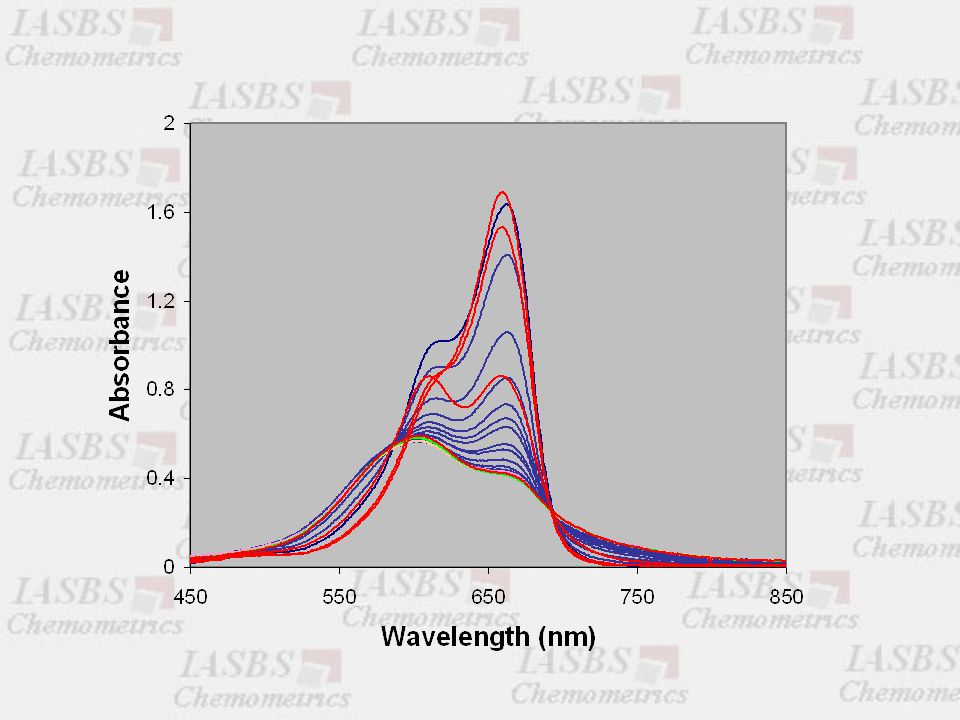
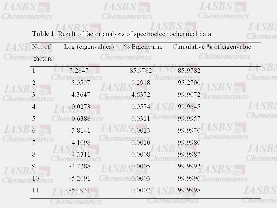
41. When iodine dissolves in a binary mixture of donating (D) and non-donating (ND) solvents, preferential solvation indicates the shape of iodine spectrum Nakanishi et al. (1987) studied the spectra of iodine in mixed binary solvents Factor analysis was used to indicate the number of component existed No extra works were reported

42. Iodine spectra in dioxane-cyclohexane

43. Iodine spectra in THF-cyclohexane

44. Eigen-values Plot

48. Dye aggregatesDye monomer Dye-Surfactant ion-pairing Pre-micelle aggregate Dye partitioned in the micelle phase

49. Absorbance Spectra of MB

51. Resolved pure spectra of the components D S-D (S-D) n D (m)

52. Concentration Profiles D S-D (S-D) n D (m)

53. D + S D-S K i = [D-S]/[D][S] n D-S (D-S) n K ag = [(D-S) n ]/[D-S] n (D-S) n n D (m) K d = [D (m) ] n /[(D-S) n ) Log K ag = log [(D-S) n ] – n log [D-S] log [(D-S) n ] = Log K ag + n log [D-S]

54. n = 4 log K ag = -0.058

56. Interaction of MO with CTAB

57. Pure spectra of MO Components D DS (DS) n D (m)

58. Concentration Profiles D (m) (DS) n

59. D DS (DS) n

60. D + S DS K i = [DS] / [D] [S] C MO = 4  10 -6 M [D] = 0.49 C MO [DS] = 0.51 C MO C S = 2.5  10 -5 M [S] = C S – [DS] K i = 4.92  10 4 4.64  10 4

62. Quinone reduction In the presence of proton source Q + e  Q  - (1) Q  - + HB  QH  + B - (2) QH  + e  QH - (3) QH - +HB  QH 2 + B - (4)

63. Our data set Vis. Spectra of 0.1 mM solution of 9,10- anthraquinone at different applied potential in DMF solution Optically transparent thin layer electrode (OTTLE) The experiment was conducted in Arak University

66. EFA Plot

67. Pure spectra 1) AQ -o 2) AQH - 3) AQ 2-

68. Concentration Profiles

69. Conversion of AQ -o to AQH - AQ -o + H +  AQH - E = E  - (0.0592/n) log ([AQH - ]/[AQ -o ][H + ]) E = E  - (0.0592/n) log(1/[H+]) - (0.0592/n) log ([AQH - ]/[AQ -o ])

70. R2 = 0.996 Slope = 0.0594 intercept = -1.37

71. MCR-ALS of polarographic data applied to the study of the copper-binding ability of tannic acid Structures of tannic acid (TA) (a) and condensed tannin (b) R. Tauler et al Anal. Chim. Acta 424 (2000) 203–209

72. DPP obtained for the system C u( I I) + TA during the titration of a 1× 1 0 - 5 mol l -1 Cu(II) solution with TA in the presence of 0.01 mol l - 1 KNO3 and 0.01 mol l - 1 acetate buffer (pH = 5. 0). The thick line denotes the polarogram measured for the metal ions in the absence of TA. Cu +2 I = CV + E Cu+2 + TA

73. Singular value decomposition (SVD) for the data repre-sented

74. Concentration profiles (a, c, e) and normalised pure voltammograms (b, d, f), in arbitrary units, obtained in the MCR-ALS decomposition of the data matrix of Fig. 2 according to different assumptions: three components with selectivity, non-negativity and unimodality constrains (a, b) (lof 8.1%); four components with selectivity, non-negativity and unimodality (c, d) (lof 4.4%) or four components with selectivity, non-negativity and signal shape (e, f) (lof 6.5%)

75. Study of the interaction equilibria between the ploynucleotide poly (inosinic)-poly(cytidilic) acid and Ethidium bromide by means of coupled spectrometric techniques R. Tauler et al. Anal. Chim. Acta 424 (2000) 105-114 poly(I)-poly(C) Ethidium bromide (EtBr) ( 3,8-diamino-5-ethyl-6- phenylphenantridinium) Activator of in vivo the interferon biosynthesis Fluorescent dye

76. poly(I)-poly(C) concentration constant EtBr concentration constant 37 o C, neutral pH, KH 2 PO 4 0.021 M, Na 2 HPO 4 0.029 M, and NaCl 0.15 M, I total =0.26 M Techniques Molecular absorption Fluorscence Circular dicroism (CD) Methods Continous variation Mole-ratio Experimental conditions

77. D UV-Vis var D fluor var D DC var D UV-Vis Et D fluor Et D DC Et D UV-Vis poly D fluor poly D DC poly

78. Data matrices arrangement: (a) analysis of a single spectroscopic data matrix; (b) simultaneous analysis of several spectroscopic data matrices corresponding to different spectroscopic techniques and different experiments.

80. C var S UV-Vis S fluor S CD C Et C pol y poly(I)-poly(C) EtBr poly(I)-poly(C)-Et Poly(I)-poly(C) + EtBr  EtBr poly complex K app = [EtBr poly complex] /[Poly(I)-poly(C) EtBr] RESULTS The intercalation sites occur every 2-3 base pairs and the value for the log Kapp was 4.6  0.1 M -1

81. R. Tauler, R. Gargallo, M. Vives and A. Izquierdo- Ridorsa Chemometrics and Intelligent Lab Systems, 1998 Study of conformational equilibria of polynucleotides

82. Poly(adenylic)-poly(uridylic) acid system Melting data Absorbance Wavelength (nm) Temperature (°C)

83. Melting data recorded at = 260 nm (univariate data analysis) Temperature (°C) Absorbance Melting Curve

84. Melting recorded at = 280 nm Temperature (°C) Absorbance Melting Curve

85. Poly(A)-poly(U) system. Two different melting experiments ALS recovered concentration profiles poly(A)-poly(U)-poly(U) ts poly(A)-poly(U) ds poly(U) rc poly(A) rc poly(A) cs Relative concentration Temperature (°C)

86. ALS recorded pure spectra