1. Least Squares Regression
D3: 3.2a
Target Goal: I can make predictions using a least square regression line.
Hw: pg 162: 27 – 32, 36, 38, 40, 42, 62

2. LSRL: least squares regression line
a model for the data
a line that summarizes the two variables
It makes the sum of the squares of the vertical distances of the data points as small as possible

3. The LSRL minimizes the total area of the squares.
The LSRL makes the sum of the squares of these distances as small as possible.
The LSRL minimizes the total area of the squares.

4. Regression Line Straight line
Describes how the response variable y changes as the explanatory variable x changes.
Use regression line to predict value of y for given value of x.
Regression (unlike correlation) requires both an explanatory and response variable.

5. The dashed line shows how to use the regression line to predict.
You can find the vertical distance of each point on the scatterplot from the regression line.

6. Predictions and Error Error (residual) = observed y – predicted ŷ
We are interested in the vertical distance of each point on the scatterplot from the regression line.
If we predict 4.9, and the actual value turns out to be 5.1, our error is the vertical distance.
Error (residual) = observed y – predicted ŷ

7. Equation of the least squares regression line
We have data on an explanatory variable x and a response variable y for n individuals.
From the data, calculate the means x bar, y bar, sx, sy of the two variables, and their correlation r.

8. The Least Squares Regression Line (LSRL):
ŷ = a + bx
with slope,
b =
and intercept,
a = y – b

9. ŷ = a + bx y: the observed value ŷ: the predicted value
every LSRL passes through
slope: rate of change
We will usually not calculate by hand, we will use the calculator.

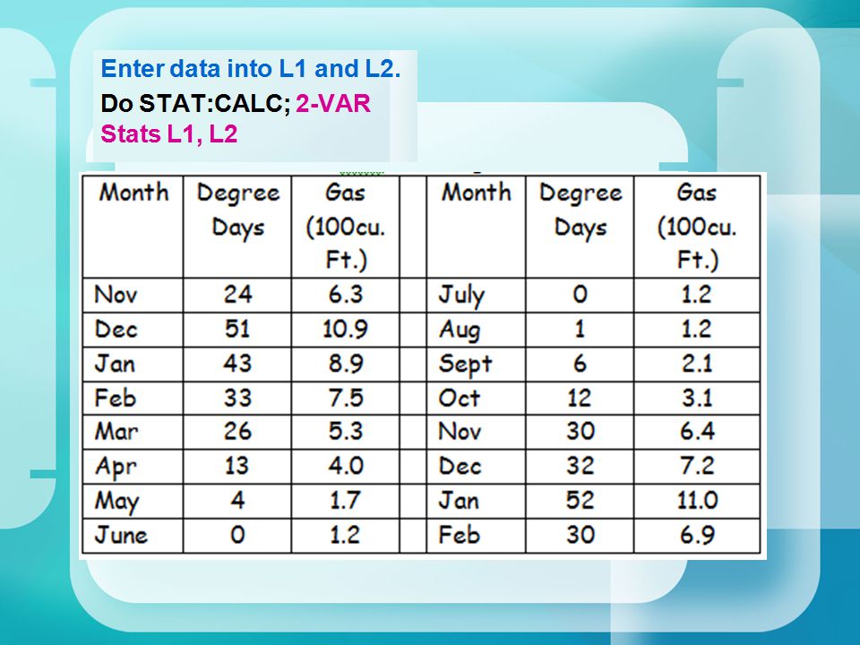
10. Exercise: Gas Consumption
The equation of the regression line of gas consumption y on the degree-days x is:
ŷ = x

11. Verifying ŷ = x
Use your calculator to find the mean and standard deviation of both x and y and their correlation r from data in the following table.

13. x bar =
= 22.31
Sx =
= 17.74
y bar =
= 5.306
Sy =
= 3.368
r =

14. Using what we’ve found, find the slope b and intercept a of the regression line from these.
This Verifies ŷ = x except for round off error.

15. Least squares lines on the calculator
Use the same data you entered into L1 and L2. (Turn off other plots & graphs.)
Define the scatterplot using L1 and L2 and the use ZoomStat to plot.

16. Press STAT:CALC:(8)LinReg(a+bx):L1,L2,Y1:enter
To enter Y1, VARS:Y-VARS:(1)FUNCTION}
If r2 and r do not appear on your screen, press 2nd:0 (catalog).
Scroll down to “DiagnosticOn” and press enter.

17. Press GRAPH to overlay the LSRL on the scatterplot.
Note: verify LSRL equation at Y1 to be
ŷ = x

18. Least-Squares Regression
Interpreting a Regression Line
Consider the regression line from the example
“Does Fidgeting Keep You Slim?” Identify the slope and y-intercept and interpret each value in context.
Least-Squares Regression
The y-intercept a = kg is the fat gain estimated by this model if NEA does not change when a person overeats.
The slope b = tells us that the amount of fat gained is predicted to go down by kg for each added calorie of NEA.

19. Least-Squares Regression
Prediction
We can use a regression line to predict the response ŷ for a specific value of the explanatory variable x.
Use the NEA and fat gain regression line to predict the fat gain for a person whose NEA increases by 400 cal when she overeats.
Least-Squares Regression
We predict a fat gain of 2.13 kg when a person with NEA = 400 calories.

20. Least-Squares Regression
Interpreting Computer Regression Output
A number of statistical software packages produce similar regression output. Be sure you can locate
the slope b,
the y intercept a,
and the values of s and r2.
Least-Squares Regression

21. The slope b = tells us that the amount of Pct is predicted to go down by units for each additional pair.
The y-intercept a = is the Pct estimated by this model when there are no pairs.