1. SIMPLE AND MULTIPLE REGRESSION

2. Relació entre variables
Entre variables discretes
(exemple: veure Titanic)
Entre continues (Regressió !)
Entre discretes i continues (Regressió!)

3. > Rendiment en Matemàtiques, > Nombre de llibres a casa
Pisa 2003
> Rendiment en Matemàtiques, > Nombre de llibres a casa

4. > Rendiment en Matemàtiques, > Nombre de llibres a casa
Pisa 2003
> Rendiment en Matemàtiques, > Nombre de llibres a casa

5. Regressió Lineal ? Pisa 2003 EXAMINE
VARIABLES=fac1_1 BY st19q01 /PLOT=BOXPLOT/STATISTICS=NONE/NOTOTAL
/MISSING=REPORT.

6. Regressió Lineal ? Pisa 2003 EXAMINE
VARIABLES=fac1_1 BY st19q01 /PLOT=BOXPLOT/STATISTICS=NONE/NOTOTAL
/MISSING=REPORT.

7. Regressió
Lineal ?
Pisa 2003
mean=c( , , , , )
books = c(1,2,3, 4, 5)
plot(books, mean, col="blue", axes=FALSE, xlab="books", ylab="level mat")
axis(1)
axis(2)
abline(lm(mean~books), col="red")

8. Regressió Lineal

9. * We first load the PISAespanya.sav file and then
* this is the sintaxis file for SPSS analysis
*Q38 How often do these things happen in your math class
*Student dont't listen to what the teacher says
CROSSTABS
/TABLES=subnatio BY st38q02
/FORMAT= AVALUE TABLES
/STATISTIC=CHISQ
/CELLS= COUNT ROW .
FACTOR
/VARIABLES pv1math pv2math pv3math pv4math pv5math pv1math1 pv2math1
pv3math1 pv4math1 pv5math1 pv1math2 pv2math2 pv3math2 pv4math2 pv5math2
pv1math3 pv2math3 pv3math3 pv4math3 pv5math3 pv1math4 pv2math4 pv3math4
pv4math4 pv5math4 /MISSING LISTWISE /ANALYSIS pv1math pv2math pv3math
pv4math pv5math pv1math1 pv2math1 pv3math1 pv4math1 pv5math1 pv1math2
pv2math2 pv3math2 pv4math2 pv5math2 pv1math3 pv2math3 pv3math3 pv4math3
pv5math3 pv1math4 pv2math4 pv3math4 pv4math4 pv5math4
/PRINT INITIAL EXTRACTION FSCORE
/PLOT EIGEN ROTATION
/CRITERIA FACTORS(1) ITERATE(25)
/EXTRACTION ML
/ROTATION NOROTATE
/SAVE REG(ALL) .
GRAPH
/SCATTERPLOT(BIVAR)=st19q01 WITH fac1_1
/MISSING=LISTWISE .
REGRESSION
/MISSING LISTWISE
/STATISTICS COEFF OUTS R ANOVA
/CRITERIA=PIN(.05) POUT(.10)
/NOORIGIN
/DEPENDENT fac1_1
/METHOD=ENTER st19q01
/PARTIALPLOT ALL
/SCATTERPLOT=(*ZRESID ,*ZPRED )
/RESIDUALS HIST(ZRESID) NORM(ZRESID) .

10. library(foreign)
help(read.spss)
data=read.spss("G:/DATA/PISAdata2003/ReducedDataSpain.sav", use.value.labels=TRUE,to.data.fram=TRUE)
names(data)
[1] "SUBNATIO" "SCHOOLID" "ST03Q01" "ST19Q01" "ST26Q04" "ST26Q05"
[7] "ST27Q01" "ST27Q02" "ST27Q03" "ST30Q02" "EC07Q01" "EC07Q02"
[13] "EC07Q03" "EC08Q01" "IC01Q01" "IC01Q02" "IC01Q03" "IC02Q01"
[19] "IC03Q01" "MISCED" "FISCED" "HISCED" "PARED" "PCMATH"
[25] "RMHMWK" "CULTPOSS" "HEDRES" "HOMEPOS" "ATSCHL" "STUREL"
[31] "BELONG" "INTMAT" "INSTMOT" "MATHEFF" "ANXMAT" "MEMOR"
[37] "COMPLRN" "COOPLRN" "TEACHSUP" "ESCS" "W.FSTUWT" "OECD"
[43] "UH" "FAC1.1"
attach(data)
mean(FAC1.1)
[1] e-16
tabulate(ST19Q01)
[1]
> table(ST19Q01)
ST19Q01
Miss Invalid N/A More than 500 books
books books books books
0-10 books
375

11. Efecto de Cultural Possession of the family

12. Data
Variables Y and X observed
on a sample of size n:
yi , xi
i =1,2, ..., n

13. Covariance and correlation

14. Scatterplot for various values of correlation
par(mfrow=c(4,4))
for (i in seq(-1,1,.2) ) {
r=i;
X =rnorm(n)
Y=r*X+ sqrt((1-r^2))*rnorm(n)
plot(X,Y, main=c("correlation", as.character(r)), col="blue")
regress= lm(Y ~X)
abline(regress) }

15. Coeficient de correlació r = 0 , tot i que hi ha una relació funcional exacta (no lineal!)
> cbind(x,y)
x y
[1,]
[2,]
[3,]
[4,]
[5,]
[6,]
[7,]
[8,]
[9,]
[10,]
[11,]
[12,]
[13,]
[14,]
[15,]
[16,]
[17,]
[18,]
[19,]
[20,]
[21,]
>
x=seq(-10,10,1)
y = x^2
r=cov(x,y)/(var(x)*var(y)) r
[1] 0
plot(x,y,col="blue", axes=FALSE)
axis(1)
axis(2)
abline(lm(y~x), col="red")

16. Regressió Lineal Simple
Variables Y X
E Y | X = a + b X
Var (Y | X ) = s2

17. Linear relation: y = 1 + .6 X ############ values of X
X = (-0.5+ runif(100))*30#### exact linear relation
alpha=1; beta=.6;
y =alpha + beta*X
#######################
plot(X,y,xlim=c(-15,15),ylim=c(-15,15),type="l", col="red", axes=FALSE,xlab="axis X", ylab="axis y")
abline(v=0)
abline(h=0)
axis(1,seq(-14,14,1),cex=.2)
axis(2,seq(-14,14,1),cex=.2)

18. Linear relation and sample data
sigma=3;
E= rnorm(length(X))
Y=y+ sigma*E
lines(X,Y,type="p", col="blue")

19. Yi = a + b Xi + ei ei : mean zero variance s2 normally distributed
Regression Model
Yi = a + b Xi + ei
ei :
mean zero
variance s2
normally distributed

20. Sample Data: Scatterplot
######## the sample data: scatterplot
plot(X,Y,xlim=c(-15,15),ylim=c(-15,15),type="p", col="blue", axes=FALSE,xlab="axis X", ylab="axis y")
abline(v=0)
abline(h=0)
axis(1,seq(-14,14,1),cex=.2)
axis(2,seq(-14,14,1),cex=.2)

21. Fitted regression line
a= b=0.6270
######## the sample data: scatterplot
plot(X,Y,xlim=c(-15,15),ylim=c(-15,15),type="p", col="blue", axes=FALSE,xlab="axis X", ylab="axis y")
abline(v=0)
abline(h=0)
axis(1,seq(-14,14,1),cex=.2)
axis(2,seq(-14,14,1),cex=.2)
abline(lm(Y~X), col=“green")

22. Fitted and true regression lines:
a= b=0.6270
a=1, b=.6
abline(c(alpha,beta),col="red")

23. Fitted and true regression lines in repeated (20) sampling
a=1, b=.6
abline(c(alpha,beta),col="red")
############ values of X
X = (-0.5+ runif(100))*30#### exact linear relation
alpha=1; beta=.6;
y =alpha + beta*X
#######################
plot(X,y,xlim=c(-15,15),ylim=c(-15,15),type="l", col="red", axes=FALSE,xlab="axis X", ylab="axis y")
abline(v=0)
abline(h=0)
axis(1,seq(-14,14,1),cex=.2)
axis(2,seq(-14,14,1),cex=.2)
for (i in 1:20) {
# Sample Data
sigma=3;
E= rnorm(length(X))
Y=y+ sigma*E
# lines(X,Y,type="p", col="blue")
abline(lm(Y~X), col="green") }
######## the sample data: scatterplot
# plot(X,Y,xlim=c(-15,15),ylim=c(-15,15),type="p", col="blue", axes=FALSE,xlab="axis X", ylab="axis y")
plot(X,Y,xlim=c(-15,15),ylim=c(-15,15),type="p", col="blue", axes=FALSE,xlab="axis X", ylab="axis y")

24. OLS estimate of beta (under repeated sampling)
Estimate of beta for different samples (100):
>
a=1, b=.6
> mean(bs)
[1]
> sd(bs)
[1]
>
############ values of X
X = (-0.5+ runif(100))*30#### exact linear relation
alpha=1; beta=.6;
y =alpha + beta*X
#######################
plot(X,y,xlim=c(-15,15),ylim=c(-15,15),type="l", col="red", axes=FALSE,xlab="axis X", ylab="axis y")
abline(v=0)
abline(h=0)
axis(1,seq(-14,14,1),cex=.2)
axis(2,seq(-14,14,1),cex=.2)
bs = c()
for (i in 1:100) {
# Sample Data
sigma=3;
E= rnorm(length(X))
Y=y+ sigma*E
# lines(X,Y,type="p", col="blue")
bs=c( bs,lm(Y ~X)$coefficients[2])
abline(lm(Y~X), col="green")
abline(c(alpha,beta),col="red") }
plot(bs, ylim=c(.3,.9), col="blue")
abline(h=.6, col="red")
mean(bs)
sd(bs)

25. REGRESSION Analysis of the Simulated Data
(with R and other software )

26. Fitted regression line:
a=1, b=.6
a= , b=
# Sample Data
sigma=3;
E= rnorm(length(X))
Y=y+ sigma*E
lines(X,Y,type="p", col="blue")
######## the sample data: scatterplot
plot(X,Y,xlim=c(-15,15),ylim=c(-15,15),type="p", col="blue", axes=FALSE,xlab="axis X", ylab="axis y")
abline(v=0)
abline(h=0)
axis(1,seq(-14,14,1),cex=.2)
axis(2,seq(-14,14,1),cex=.2)
############## fitted regression line
b= sum((Y-mean(Y))*(X - mean(X)))/ sum( (X - mean(X))^2)
a = mean(Y) - b*mean(X)
abline(c(a,b),col= "green")
abline(c(alpha,beta),col="red")
c(a,b)

27. Regression Analysis regression = lm(Y ~X) summary(regression) Call:
lm(formula = Y ~ X)
Residuals:
Min Q Median Q Max
Coefficients:
Estimate Std. Error t value Pr(>|t|)
(Intercept) **
X < 2e-16 ***
---
Signif. codes: 0 `***' `**' 0.01 `*' 0.05 `.' 0.1 ` ' 1
Residual standard error: on 98 degrees of freedom
Multiple R-Squared: , Adjusted R-squared:
F-statistic: on 1 and 98 DF, p-value: < 2.2e-16
>>
regression = lm(Y ~X)
summary(regression)

28. Regression Analysis with Stata
. use "E:\Albert\COURSES\cursDAS\AS2003\data\MONT.dta", clear
. regress y x
Source | SS df MS Number of obs =
F( 1, 98) =
Model | Prob > F =
Residual | R-squared =
Adj R-squared =
Total | Root MSE =
y | Coef. Std. Err t P>|t| [95% Conf. Interval]
x |
_cons |
. predict yh
. graph yh y x, c(s.) s(io)

29. Regression analysis with SPSS

30. Estimación

31. Gráfico de dispersión

32. Fitted Regression FYi = 1.02 + .64 Xi , R2=.74 s.e.: (.037)
t-value:
Regression coeficient of X is significant (5% significance level),
with the expected value of Y icreasing .64 for each unit increase of X. The 95% confidence interval for the regression coefficient is
[ *.037, *.037]=[.57, .71]
74% of the variation of Y is explained by the variation of X

33. Fitted regression line
graph yh y x, c(s.) s(io)

34. Residual plot
. graph e x, yline(0)

35. OLS analysis

36. Variance decomposition

37. Properties of OLS estimation

38. Sampling distributions

39. Inferences

40. Student-t distribution

41. Significance tests

42. F-test

43. Prediction of Y

44. Multiple Regression:

45. t-test and CI

46. F-test

47. Confidence bounds for Y

48. Interpreting multiple regression by means of simple regression

49. Adjusted R2

50. Exemple de l’Anàlisi de Regressió
Dades de paisos.sav

51. Variables

52. Matrix Plot
Necessitat de transformar les variables !

53. Transformació de variables

54. Matrix Plot
Relacions (aproximadament) lineals entre variables transformades !

55. Anàlisi de Regressió REGRESSION /MISSING LISTWISE
/STATISTICS COEFF OUTS R ANOVA
/CRITERIA=PIN(.05) POUT(.10)
/NOORIGIN
/DEPENDENT espvida
/METHOD=ENTER calories logpib logmetg
/PARTIALPLOT ALL
/SCATTERPLOT=(*ZRESID ,*ZPRED )
/SAVE RESID .

56. Residus vs y ajustada:

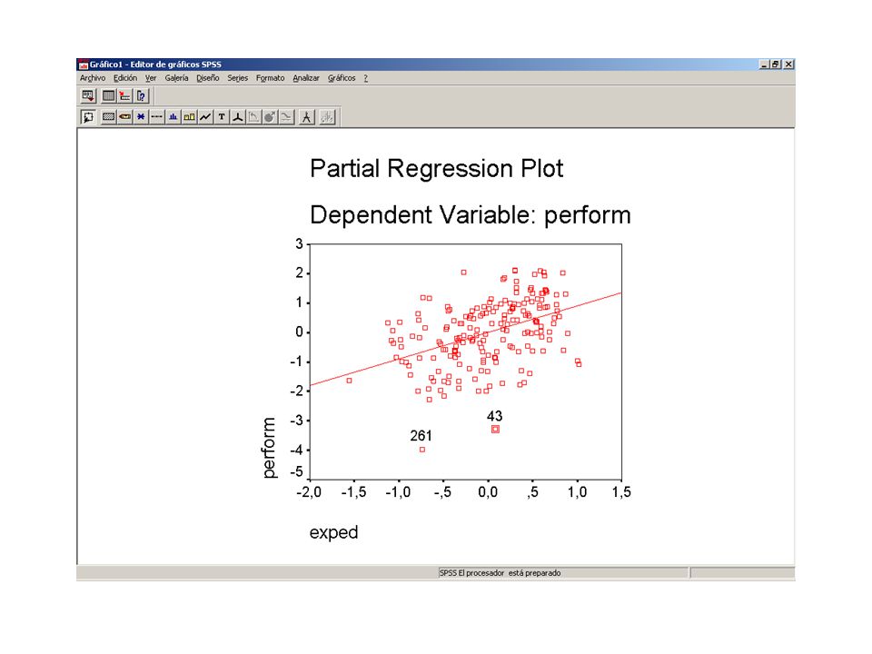
57. Regressió parcial:

58. Regressió parcial:

59. Regressió parcial

60. Anàlisi de Regressió REGRESSION /MISSING LISTWISE
/STATISTICS COEFF OUTS R ANOVA
/CRITERIA=PIN(.05) POUT(.10)
/NOORIGIN
/DEPENDENT espvida
/METHOD=ENTER calories logpib logmetg cal2
/PARTIALPLOT ALL
/SCATTERPLOT=(*ZRESID ,*ZPRED )
/SAVE RESID .

61. Residus vs y ajustada

62. Case missfit Potential for influence: Leverage Influence
Case statistics
Case missfit
Potential for influence: Leverage
Influence

63. Residuals

64. Hat matrix

65. Influence Analysis

66. Diagnostic case statistics
After fitting regression, use the instruction
Fpredict namevar
predicted value of y
, cooksd Cook’s D influence measure
, dfbeta(x1) DFBETAS for regression coefficient on var x1
, dfits DFFITS influence measures
, hat Diagonal elements of hat matrix (leverage)
, leverage (same as hat)
, residuals
, rstandard standardized residuals
, .rstudent Studentized residuals
, stdf standard erros of predicte individual y, standard error of forecast
, stdp standard errors of predicted mean y
, stdr standard errors of residuals
, welsch Welsch’s distance influence measure
display tprob(47, 2.337)
Sort namevar
list x1 x2 –5/1

67. Leverages after fit … . fpredict lev, leverage . gsort -lev
. list nombre lev in 1/5
nombre lev
RECAGUREN SOCIEDAD LIMITADA,
EL MARQUES DEL AMPURDAN S,L,
ADOBOS Y DERIVADOS S,L,
CONSERVAS GARAVILLA SA
5. PLANTA DE ELABORADOS ALIMENTICIOS MA .

68. Box plot of leverage values
. predict lev, leverage
. graph lev, box s([_n])
Cases with extreme leverages

69. Leverage versus residual square plot
. lvr2plot, s([_n])

70. Dfbeta’s:
. fpredict beta, dfbeta(nt_paau)
. graph beta, box s([_n])

71. Regression: Outliers, basic idea

72. Regression: Outliers, indicators
Description
Rule of thumb (when “wrong”)
Resid
Residual: actual – predicted -
ZResid
Standardized residual: residual divided by standarddeviation residual
> 3 (in absolute value)
SResid
Studentized Residu: residual divided by standarddeviation residual at that particular datapoint of X values
DResid
Difference residual and residual when datapoint deleted
SDResid
See DResid, standardized by standard deviation at that particular datapoint of X values

73. Regression: Outliers, in SPSS

74. Regression: Influential Points, Basic Idea
Influential Point (no outlier!)

75. Regression: Influential Points, Indicators
Description
Rule of thumb
Lever
Afstand tussen punt en overige punten NB: potentieel invloedrijk
> 2 (p+1) / n
Cook
Verandering in residuen van overige cases als een bepaalde case niet in de regressie meedoet
> 1
DfBeta
Verschil tussen beta’s wanneer de case wel meedoet en wanneer die niet meedoet in het model NB: voor elke beta krijgen we deze -
SdfBeta
DfBeta / Standaardfout DfBeta NB: voor elke beta
> 2/√n
DfFit
Verschil tussen voorspelde waarde als case wel versus niet meedoet in model
SDfFit
DfFit / standaarddeviatie SdFit
> 2 /√(p/n)
CovRatio
Verandering in Varianties/Covarianties als punt niet meedoet
Abs (CovRatio – 1)> 3 p / n

76. Regression: Influential points, in SPSS
Case 2 is an influential point

81. Regression: Influential Points, what to do?
Nothing at all..
Check data
Delete a-typical datapoints, then repeat regression without these datapoints
“to delete a point or not is an issue statisticians disagree on”

82. MULTICOLLINEARITY
Diagnostic tools

83. Regression: Multicollinearity
If predictors correlate “high”, then we speak of multicollinearity
Is this a problem? If you want to asess the influence of each predictor, yes it is, because:
Standarderrors blow up, making coefficients not-significant

84. Analyzing math data
. use "G:\Albert\COURSES\cursDAS\AS2003b\data\mat.dta", clear
. save "G:\Albert\COURSES\CursMetEstad\Curs2004\Metodes\mathdata.dta"
file G:\Albert\COURSES\CursMetEstad\Curs2004\Metodes\mathdata.dta saved
. edit
- preserve
. gen perform = (nt_m1+ nt_m2+ nt_m3)/3
(110 missing values generated)
. corr perform nt_paau nt_acces nt_exp
(obs=189)
| perform nt_paau nt_acces nt_exp
perform |
nt_paau |
nt_acces |
nt_exp |
. outfile nt_exp nt_paau nt_acces perform using "G:\Albert\COURSES\CursMetEsta
> d\Curs2004\Metodes\mathdata.dat" .

86. Multiple regression: perform vs nt_acces nt_paau
. regress perform nt_acces nt_paau
Source | SS df MS Number of obs =
F( 2, 242) =
Model | Prob > F =
Residual | R-squared =
Adj R-squared =
Total | Root MSE =
perform | Coef. Std. Err t P>|t| [95% Conf. Interval]
nt_acces |
nt_paau |
_cons | .
Perform = rendiment a mates I a III

87. Collinearity

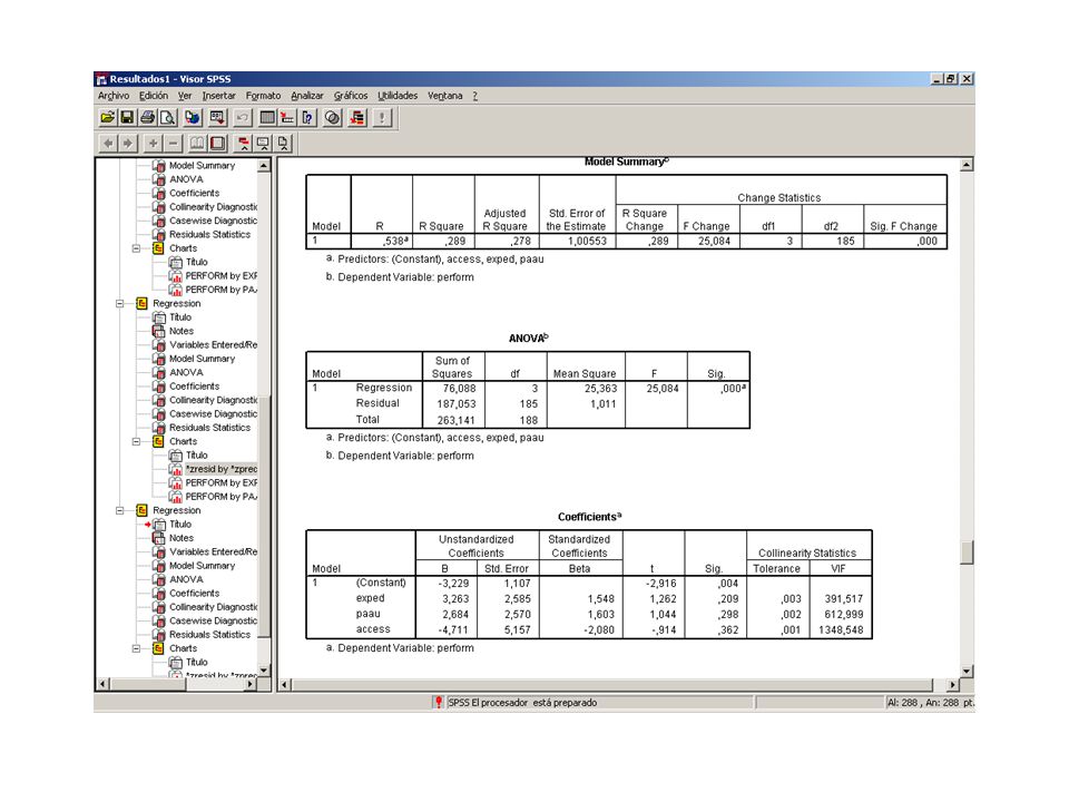
88. Diagnostics for multicollinearity
. corre nt_paau nt_exp nt_acces
(obs=276)
| nt_paau nt_exp nt_acces
nt_paau|
nt_exp|
nt_acces|
. fit perform nt_paau nt_exp nt_access
. vif
Variable | VIF /VIF
nt_acces |
nt_paau |
nt_exp |
Mean VIF | .
VIF = 1/(1 – Rj2)
Any explanatory variable with a
VIF greater than 5 (or tolerance
less than .2) show a degree
of collinearity that may be
Problematic
This ratio is called Tolerance
In the case of just nt_paau an nt_exp we
Get
. vif
Variable | VIF /VIF
nt_exp |
nt_paau |
Mean VIF | .

89. Multiple regression: perform vs nt_paau nt_exp
. regress perform nt_paau nt_exp
Source | SS df MS Number of obs =
F( 2, 186) =
Model | Prob > F =
Residual | R-squared =
Adj R-squared =
Total | Root MSE =
perform | Coef. Std. Err t P>|t| [95% Conf. Interval]
nt_paau |
nt_exp |
_cons |
. corr nt_exp nt_paau nt_acces
(obs=276)
| nt_exp nt_paau nt_acces
nt_exp |
nt_paau |
nt_acces |
. predict yh
(option xb assumed; fitted values)
(82 missing values generated)
. predict e, resid
(169 missing values generated) .

90. Regression: Multicollinearity, Indicators
description
Rule of thumb (when “wrong”)
Overall F_Test versus test coefficients
Overall F-Test is significant, but individual coefficients are not -
Beta
Standardized coefficient
Outside [-1, +1]
Tolerance
Tolerance = unique variance of a predictor (not shared/explained by other predictors) … NB: Tolerance per coefficient
< 0.01
Variantie Inflation Factor
√ VIF indicates how much the standard error of a particular coefficient is inflated due to correlatation between this particular predictor and the other predictors
NB: VIF per coefficient
>10
Eigenvalues
…rather technical…
+/- 0
Condition Index
> 30
Variance Proportion
…rather technical…look tot “loadings” on the dimensions
Loadings around 1

91. Regression: Multicollinearity, in SPSS
diagnostics

92. Regression: Multicollineariteit, in SPSS
Beta > 1
Tolerance, VIF in orde

93. Regressie: Multicollineariteit, in SPSS
2 eigenwaarden rond 0
CI in orde
Deze variabelen zorgen voor multicoll.

94. Regression: Multicollinearity, what to do?
Nothing… (if there is no interest in the individual coefficients, only in good prediction)
Leave one (or more) predictor(s) out
Use PCA to reduce high correlated variables to smaller number of uncorrelated variables

95. Variables Categòriques
Use: Survey_sample.sav, in i/.../data

96. Salari vs gènere | anys d’educació status de treball

97. Creació de variables dicotòmiques
GET
FILE='G:\Albert\Web\Metodes2005\Dades\survey_sample.sav'.
COMPUTE D1 = wrkstat=1.
EXECUTE .
COMPUTE D2 = wrkstat=2.
COMPUTE D3 = wrkstat=3.
COMPUTE D4 = wrkstat=4.
COMPUTE D5 = wrkstat=5.
COMPUTE D6 = wrkstat=6.
COMPUTE D7 = wrkstat=7.
COMPUTE D8 = wrkstat=8.

98. Regressió en blocks REGRESSION /MISSING LISTWISE
/STATISTICS COEFF OUTS R ANOVA CHANGE
/CRITERIA=PIN(.05) POUT(.10)
/NOORIGIN
/DEPENDENT rincome
/METHOD=ENTER sex
/METHOD=ENTER d2 d3 d4 d5 d6 d7 d8 .

100. Regressió en blocks REGRESSION /MISSING LISTWISE
/STATISTICS COEFF OUTS R ANOVA CHANGE
/CRITERIA=PIN(.05) POUT(.10)
/NOORIGIN
/DEPENDENT rincome
/METHOD=ENTER sex
/METHOD=ENTER educ
/METHOD=ENTER d2 d3 d4 d5 d6 d7 d8 .

101. Categorical Predictors
Is income dependent on years of age and religion ?

102. Categorical Predictors
Compute dummy variable for each category, except last

103. Categorical Predictors
And so on…

104. Categorical Predictors
Block 1

105. Categorical Predictors
Block 2

106. Categorical Predictors
Ask for R2 change

107. Categorical Predictors
Look at R Square change for importance of categorical variable