1. Structural Equation Modeling Using Mplus Chongming Yang Research Support Center FHSS College

2. Structural? Structuralism Structuralism Components Components Relations Relations

3. Objectives Introduction to SEM Introduction to SEM The model The model Parameters Parameters Estimation Estimation Model evaluation Model evaluation Applications Applications Estimate simple models with Mplus Estimate simple models with Mplus

4. Continuous Dependent Variables Session I

5. Information of Variable Mean Mean Variance Variance Skewedness Skewedness Kurtosis Kurtosis

6. Variance & Covariance

7. Covariance Matrix (S) x1 x2 x3 x1 x2 x3 x1 V 1 x2 Cov 21 V 2 x3 Cov 31 Cov 32 V 3

8. Statistical Model Probabilistic statement about Relations of variables Probabilistic statement about Relations of variables Imperfect but useful representation of reality Imperfect but useful representation of reality

9. Structural Equation Modeling A system of regression equations for latent variables to estimate and test direct and indirect effects without the influence of measurement errors. A system of regression equations for latent variables to estimate and test direct and indirect effects without the influence of measurement errors. To estimate and test theories about interrelations among observed and latent variables. To estimate and test theories about interrelations among observed and latent variables.

10. Latent Variable ( Construct / Factor / Trait ) A hypothetical variable A hypothetical variable cannot be measured directly cannot be measured directly No objective measurement unit No objective measurement unit inferred from observable manifestations inferred from observable manifestations Multiple manifestations (indicators) Multiple manifestations (indicators) Normally distributed interval dimension Normally distributed interval dimension

11. How is Depression Distributed in? BYU students BYU students Patients for Therapy Patients for Therapy

12. Normal Distributions

13. Levels of Analyses Observed Observed Latent Latent

14. Test Theories Classical True Score Theory: Classical True Score Theory: Observed Score = True score + Error Observed Score = True score + Error Item Response Theory Item Response Theory Generalizability (Raykov & Marcoulides, 2006) Generalizability (Raykov & Marcoulides, 2006)

15. Graphic Symbols of SEM Rectangle – observed variable Rectangle – observed variable Oval -- latent variable or error Oval -- latent variable or error Single-headed arrow -- causal relation Single-headed arrow -- causal relation Double-headed arrow -- correlation Double-headed arrow -- correlation

16. Graphic Measurement Model of Latent   X1X1 X2X2 X3X3 11 22 33 1 2 3

17. Equations Specific equations Specific equations X 1 = 1  +  1 X 2 = 2  +  2 X 3 = 3  +  3 Matrix Symbols Matrix Symbols X =  +  True Score Theory? True Score Theory?

18. Relations of Variances V X1 = 1 2 +  1 V X2 = 2 2 +  2 V X3 = 3 2 +  3  = measurement error / uniqueness

19. Unknown Parameters V X1 = 1 2 +  1 V X2 = 2 2 +  2 V X3 = 3 2 +  3

20. Sample Covariance Matrix (S) x1 x2 x3 x1 x2 x3 x1 V 1 x2 Cov 21 V 2 x3 Cov 31 Cov 32 V 3

21. Variance of  Variance of  = common covariance of X1 X2 and X3 Variance of  = common covariance of X1 X2 and X3 Variance of  11 22 33 0 0 0

22. Unstandardized Parameterization (scaling) 1 = 1 (set variance of X1 =1; X1 called reference Indicator) 1 = 1 (set variance of X1 =1; X1 called reference Indicator) Variance of  = common variance of X1 X2 and X3 Variance of  = common variance of X1 X2 and X3 Squared = explained variance of X (R 2 ) Squared = explained variance of X (R 2 ) Variance of  = unexplained variance-- error Variance of  = unexplained variance-- error Total Variance = Squared +  Variance Total Variance = Squared +  Variance

23. Just Identified Model  X1X1 X2X2 X3X3 11 22 33 1 2 3

24. Reference Indicator (marker) Choose conceptually the best Choose conceptually the best Small variance  non-convergence Small variance  non-convergence Different markers  different parameters estimates and their standard errors Different markers  different parameters estimates and their standard errors Affect measurement invariance tests Affect measurement invariance tests Not affect standardized estimates Not affect standardized estimates

25. Standardized Parameterizations (scaling) Variance of  = 1 = common variance of X1 X2 and X3 Variance of  = 1 = common variance of X1 X2 and X3 Squared = explained variance of X (R 2 ) Squared = explained variance of X (R 2 ) Variance of  = 1 - 2 Variance of  = 1 - 2 Mean of  = 0 Mean of  = 0 Mean of  = 0 Mean of  = 0

26. Two Kinds of Parameters Fixed at 0, 1, or other values Fixed at 0, 1, or other values Freely estimated Freely estimated

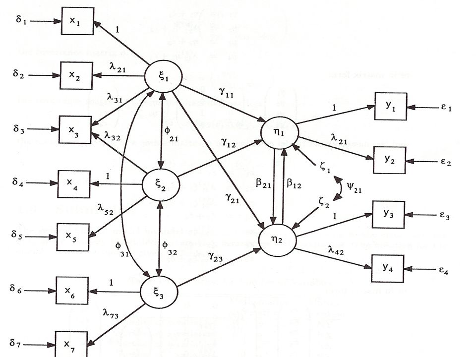
30. Structural Equation Model in Matrix Symbols X = x  +  (exogenous) X = x  +  (exogenous) Y = y  +  (endogenous) Y = y  +  (endogenous)  =  +  +  (structural model)  =  +  +  (structural model) Note: Measurement model reflects the true score theory

31. Structural Equation Model in Matrix Symbols X =  x + x  +  (measurement) X =  x + x  +  (measurement) Y =  y + y  +  (measurement) Y =  y + y  +  (measurement)  = α +  +  +  (structural)  = α +  +  +  (structural) Note: SEM with mean structure.

32. Model Implied Covariance Matrix (Σ) Note: This covariance matrix contains unknown parameters in the equations. (I-B) = non-singular

33. Estimations/Fit Functions Hypothesis:  = S or  - S = 0 Hypothesis:  = S or  - S = 0 Maximum Likelihood Maximum Likelihood F = log||  || + trace(S  -1 ) - log||S|| - (p+q) F = log||  || + trace(S  -1 ) - log||S|| - (p+q)

34. Convergence -- Reaching Limit Minimize F while adjust unknown Parameters through iterative process Minimize F while adjust unknown Parameters through iterative process Convergence value: F difference between last two iterations Convergence value: F difference between last two iterations Default convergence =.0001 Default convergence =.0001 Increase to help convergence ( 0.001 or 0.01 ) Increase to help convergence ( 0.001 or 0.01 ) e.g. Analysis: convergence =.01; e.g. Analysis: convergence =.01;

35. No Convergence No unique parameter estimates No unique parameter estimates Lack of degrees of freedom  under identification Lack of degrees of freedom  under identification Variance of reference indicator too small Variance of reference indicator too small Fixed parameters are left to be freely estimated Fixed parameters are left to be freely estimated Misspecified model Misspecified model

36. Absolute Fit Index  2 = F(N-1) (N = sample size) df = p(p+1)/2 – q P = number of variances, covariances, & means q = number of unknown parameters to be estimated prob = ? (Nonsignificant  2 indicates good fit, Why?)

37. Sample Information x1 x2 x3 x4 … x1 x2 x3 x4 … x1 v 1 x2 cov 21 v 2 x3 cov 31 cov 32 v 3 x4 cov 41 cov 42 cov 43 v 4 … … Mean1 Mean2 Mean3 Mean4 … Mean1 Mean2 Mean3 Mean4 … Total info = P(P+1)/2 + Means

38. Absolute Fit -- SRMR Standardized Root Mean Square Residual Standardized Root Mean Square Residual SRMR = Difference between observed and implied covariances in standardized metric SRMR = Difference between observed and implied covariances in standardized metric Desirable when <.90, but no consensus Desirable when <.90, but no consensus

39. Relative Fit: Relative to Baseline (Null) Model All unknown parameters are fixed at 0 All unknown parameters are fixed at 0 Variables not related ( =  =  =  =0) Variables not related ( =  =  =  =0) Model implied covariance  = 0 Model implied covariance  = 0 Fit to sample covariance matrix S Fit to sample covariance matrix S Obtain  2, df, prob <.0000 Obtain  2, df, prob <.0000

40. Relative Fit Indices CFI = 1- (  2 -df)/(  2 b -df b ) CFI = 1- (  2 -df)/(  2 b -df b ) b = baseline model b = baseline model Comparative Fit Index, desirable =>.95; 95% better than b model Comparative Fit Index, desirable =>.95; 95% better than b model TLI = (  2 b /df b -  2 /df) / (  2 b /df b -1) TLI = (  2 b /df b -  2 /df) / (  2 b /df b -1) (Tucker-Lewis Index, desirable =>.90) (Tucker-Lewis Index, desirable =>.90) RMSEA = √(  2 -df)/(n*df) RMSEA = √(  2 -df)/(n*df) (Root Mean Square of Error Approximation, desirable <=.06 (Root Mean Square of Error Approximation, desirable <=.06 penalize a large model with more unknown parameters) penalize a large model with more unknown parameters)

41. Special Case A

42. Special Cases A Assumption: x =  Assumption: x =  y =  x +  +  y =  x +  +   =  +  x +   =  +  x + 

43. Special Case B

44. Special Cases B Assumption: y =  Assumption: y =  x =  x + x  +  x =  x + x  +  y =  +   +  y =  +   + 

45. Other Special Cases of SEM Confirmatory Factor Analysis (measurement model only) Confirmatory Factor Analysis (measurement model only) Multiple & Multivariate Regression Multiple & Multivariate Regression ANOVA / MANOVA (multigroup CFA) ANOVA / MANOVA (multigroup CFA) ANCOVA ANCOVA Path Analysis Model (no latent variables) Path Analysis Model (no latent variables) Simultaneous Econometric Equations… Simultaneous Econometric Equations… Growth Curve Modeling Growth Curve Modeling …

46. EFA vs. CFA

47. Multiple Regression

48. ANCOVA

49. Multivariate Normality Assumption Observed data summed up perfectly by covariance matrix S (+ means M), S thus is an estimator of the population covariance  Observed data summed up perfectly by covariance matrix S (+ means M), S thus is an estimator of the population covariance 

50. Consequences of Violation Inflated  2 & deflated CFI and TLI  reject plausible models Inflated  2 & deflated CFI and TLI  reject plausible models Inflated standard errors  attenuate factor loadings and relations of latent variables (structural parameters) Inflated standard errors  attenuate factor loadings and relations of latent variables (structural parameters) (Cause: Sample covariances were underestimated)

51. Accommodating Strategies Accommodating Strategies Correcting Fit Correcting Fit Satorra-Bentler Scaled  2 & Standard Errors (estimator = mlm; in Mplus) Satorra-Bentler Scaled  2 & Standard Errors (estimator = mlm; in Mplus) Correcting standard errors Correcting standard errors Bootstrapping Bootstrapping Transforming Nonnormal variables Transforming Nonnormal variables Transforming into new normal indicators (undesirable) Transforming into new normal indicators (undesirable) SEM with Categorical Variables SEM with Categorical Variables

52. Satorra-Bentler Scaled  2 & SE S-B  2 = d -1 (ML-based  2 ) (d= Scaling factor that incorporates kurtosis) S-B  2 = d -1 (ML-based  2 ) (d= Scaling factor that incorporates kurtosis) Effect: performs well with continuous data in terms of  2, CFI, TLI, RMSEA, parameter estimates and standard errors. Effect: performs well with continuous data in terms of  2, CFI, TLI, RMSEA, parameter estimates and standard errors. also works with certain-categorical variables (See next slide) also works with certain-categorical variables (See next slide) Analysis: estimator = MLM;

53. Workable Categorical Data

54. Nonworkable Categorical Data

55. Bootstrapping (resampling of data) Original btstrp1 btstrp2 … Original btstrp1 btstrp2 … x y x y x y x y x y x y 1 5 5 3 1 3 1 5 5 3 1 3 2 4 1 1 5 4 2 4 1 1 5 4 3 3 3 2 4 1 3 3 3 2 4 1 4 2 4 5 2 2 4 2 4 5 2 2 5 1 2 4 3 5 5 1 2 4 3 5............

56. Limitation of Bootstrapping Assumption: Sample = Population Assumption: Sample = Population Useful Diagnostic Tool Useful Diagnostic Tool Does not Compensate for Does not Compensate for small or unrepresentative samples small or unrepresentative samples severely non-normal or severely non-normal or absence of independent samples for the cross- validation absence of independent samples for the cross- validation Analysis: Bootstrap = 500 (standard/residual); Analysis: Bootstrap = 500 (standard/residual); Output: stand cinterval; Output: stand cinterval;

57. Mplus www.statmodel.com www.statmodel.com www.statmodel.com

58. Multiple Programs Integrated SEM of both continuous and categorical variables SEM of both continuous and categorical variables Multilevel modeling Multilevel modeling Mixture modeling (identify hidden groups) Mixture modeling (identify hidden groups) Complex survey data modeling (stratification, clustering, weights) Complex survey data modeling (stratification, clustering, weights) Modern missing data treatment Modern missing data treatment Monte Carlo Simulations Monte Carlo Simulations

59. Types of Mplus Files Data (*.dat, *.txt) Data (*.dat, *.txt) Input (specify a model, <=80 columns/line) Input (specify a model, <=80 columns/line) Output (automatically produced) Output (automatically produced) Plot (automatically produced) Plot (automatically produced)

60. Data File Format Free Free Delimited by tab, space, or comma Delimited by tab, space, or comma All missing values must be flagged with special numbers / symbols All missing values must be flagged with special numbers / symbols Default in Mplus Default in Mplus Computationally slow with large data set Computationally slow with large data set Fixed Fixed Format = 3F3, 5F3.2, F5.1; Format = 3F3, 5F3.2, F5.1;

61. Mplus Input DATA: File = ? DATA: File = ? VARIABLE: Names=?; Usevar=?; Categ=?; VARIABLE: Names=?; Usevar=?; Categ=?; ANALYSIS: Type = ? ANALYSIS: Type = ? MODEL: (BY, ON, WITH) MODEL: (BY, ON, WITH) OUTPUT: Stand; OUTPUT: Stand;

62. Model Specification in Mplus BY  Measured by (F by x1 x2 x3 x4) BY  Measured by (F by x1 x2 x3 x4) ON  Regressed on (y on x) ON  Regressed on (y on x) WITH  Correlated with (x with y) WITH  Correlated with (x with y) XWITH  Interact with (inter | F1 xwith F2) XWITH  Interact with (inter | F1 xwith F2) PON  Pair ON (y1 y2 on x1 x2 = y1 on x1; y2 on x2) PON  Pair ON (y1 y2 on x1 x2 = y1 on x1; y2 on x2) PWITH  pair with (x1 x2 with y1 y2 = x1 with y1; y1 with y2) PWITH  pair with (x1 x2 with y1 y2 = x1 with y1; y1 with y2)

63. Default Specification Error or residual (disturbance) Covariance of exogenous variables in CFA Certain covariances of residuals (z2)

64. Graphic Model

65. Model Specification Model: Model: f1 by y1-y3; f2 by y4-y6; f3 by y7-y9; f4 by y10-y12; f5 by y13-y15; f5 by y13-y15; f3 on f1 f2; f4 on f2; f5 on f2 f3 f4 ; f5 on f2 f3 f4 ; MeaErrors are au

66. Practice Prepare two data files for Mplus Prepare two data files for Mplus Mediation.sav Mediation.sav Aggress.sav Aggress.sav Model Specification Model Specification Single Group CFA Single Group CFA Examine Mediation Effects in a Full SEM Examine Mediation Effects in a Full SEM Run a MIMIC model of aggressions Run a MIMIC model of aggressions Multigroup CFA to examine measurement invariance Multigroup CFA to examine measurement invariance

67. SPSS Data Missing Values? Missing Values? Leave as blank to use fixed format Leave as blank to use fixed format Recode into special number to use free format Recode into special number to use free format Save as & choose file type Save as & choose file type Fixed ASCII Fixed ASCII Free *.dat (with or without variable names?) Free *.dat (with or without variable names?) Copy & paste variable names into Mplus input file Copy & paste variable names into Mplus input file

68. Mplus Interface Activate Mplus Program Activate Mplus Program Language Generator Language Generator Manually Create An Input File Manually Create An Input File

69. Four Separate Files (Mplus) Data Data best prepared with other programs best prepared with other programs Input Input Need manually specify a model Need manually specify a model Output Output automatic output window automatic output window Graph Graph automatic graph file automatic graph file

70. Data File Individual Case Data (*.dat or *.txt) Individual Case Data (*.dat or *.txt) Free Format (default) Free Format (default) Variable separated by tab, comma, or space Variable separated by tab, comma, or space All missing values must be flagged with special symbols or numbers). All missing values must be flagged with special symbols or numbers). Fixed Format Fixed Format Variable takes fixed space, e.g. 2F2, 4F6, 5F6.3 Variable takes fixed space, e.g. 2F2, 4F6, 5F6.3 Missing values can be left blank Missing values can be left blank Summary Data Summary Data Variance-Covariance matrix, means Variance-Covariance matrix, means Correlation matrix, standard deviation, means Correlation matrix, standard deviation, means

71. SPSS  Mplus Open “Antisocial.sav” with SPSS Open “Antisocial.sav” with SPSS Work in Variable Window Work in Variable Window Option 1: Fixed Format Option 1: Fixed Format Change Format to Simplify Change Format to Simplify Save as ? (Type=Fixed ASCII ) Save as ? (Type=Fixed ASCII ) Option 2: Free Format Option 2: Free Format Recode missing values Recode missing values Save as ? (Tab-delimited) Save as ? (Tab-delimited)

72. Fixed Format F3 4F3.2 25F1 F3 4F3.2 25F1 F3  One variable that takes 3 columns F3  One variable that takes 3 columns 4F3.2  4 variables, each has 3 column 4F3.2  4 variables, each has 3 column with 2 decimals with a column with 2 decimals with a column 25F1  25 variables, each uses on 25F1  25 variables, each uses on column column

73. Copy SPSS Variable Names into Mplus Menu: Utilities  Menu: Utilities  Variables  Variables  Highlight to select variables  Highlight to select variables  Paste  Paste  Go to Syntax Window  Go to Syntax Window  Select & Copy  Select & Copy  Paste under Names Are in Mplus input file Paste under Names Are in Mplus input file Practice now Practice now

74. SAS  Mplus Assign flags to missing values (use Array code for many variables) Assign flags to missing values (use Array code for many variables) Proc Export Data = Data File Proc Export Data = Data File Outfile = “Mplus input file folder\*.dat” Outfile = “Mplus input file folder\*.dat” DBMS = dlm Replace; DBMS = dlm Replace; Run; Run; Practice Practice

75. Fixed Format Out of SAS Open with SPSS Open with SPSS Save as Fixed Format Save as Fixed Format Practice Practice

76. Stata2mplus Converting a stata data file to *.dat Converting a stata data file to *.dat Find out: http://www.ats.ucla.edu/stat/stata/faq/stata 2mplus.htm http://www.ats.ucla.edu/stat/stata/faq/stata 2mplus.htm

77. Modification Indices Lower bound estimate of the expected chi square decrease Lower bound estimate of the expected chi square decrease Freely estimating a parameter fixed at 0 Freely estimating a parameter fixed at 0 MPlus  Output: stand Mod(10); MPlus  Output: stand Mod(10); Start with least important parameters (covariance of errors) Start with least important parameters (covariance of errors) Caution: justification? Caution: justification?

78. Indirect (Mediation) Effect A*B A*B Mplus specification: Mplus specification: Model Indirect: DV IND Mediator IV;

79. Model Comparison Model: Model: Probabilistic statement about the relations of variables Probabilistic statement about the relations of variables Imperfect but useful Imperfect but useful Models Differ: Models Differ: Different Variables and Different Relations Different Variables and Different Relations (, , ,  ) (, , ,  ) Same Variables but Different Relations Same Variables but Different Relations (, , ,  ) (, , ,  )

80. Nested Model A Nested Model (b) comes from general Model (a) by A Nested Model (b) comes from general Model (a) by Removing a parameter (e.g. a path) Removing a parameter (e.g. a path) Fixing a parameter at a value (e.g. 0) Fixing a parameter at a value (e.g. 0) Constraining parameter to be equal to another Constraining parameter to be equal to another Both models have the same variables Both models have the same variables

81. Test If A=B

82. Model Comparison via  2 Difference  2 = df = (Nested model)  2 = df = (Nested model)  2 = df = (Default model)  2 = df = (Default model)___________________________________  2 dif = df dif = p = ? (a single tail)  2 dif = df dif = p = ? (a single tail) Find p value at the following website: http://www.tutor-homework.com/statistics_tables/statistics_tables.html Conclusion: If p >.05, there is no difference between the default model and nested model. Or the Hypothesis that the parameters of the two models are equal is not supported. If p >.05, there is no difference between the default model and nested model. Or the Hypothesis that the parameters of the two models are equal is not supported.

83. Practice Test if effect A=B Test if effect A=B

84. Equality Constraints in Mplus Parameter Labels: Parameter Labels: Numbers Numbers Letters Letters Combination of numbers of letters Combination of numbers of letters Constraint (B=A) Constraint (B=A) F3 on F1 (A); F3 on F1 (A); F3 on F2 (A); F3 on F2 (A);

85. Run CFA with Real Data

86. Multigroup Analysis VARIABLE: USEVAR = X1 X2 X3 X4; USEVAR = X1 X2 X3 X4; Grouping IS sex (0=F 1=M); Grouping IS sex (0=F 1=M); ANALYSIS: TYPE = MISSING H1; MODEL: F1 BY X1 - X4; F1 BY X1 - X4; MODEL M: F1 BY X2 - X4; F1 BY X2 - X4; Note: sex is grouping variable and is not used in the model.

87. Why Measurement Invariance Matters? X g1 =  g1 + g1  g1 +  g1 X g1 =  g1 + g1  g1 +  g1 X g2 =  g2 + g2  g2 +  g2 X g2 =  g2 + g2  g2 +  g2 X g1 - X g2 = (  g1 -  g2 ) + ( g1  g1 - g2  g2 ) + (  g1 -  g2 ) X g1 - X g2 = (  g1 -  g2 ) + ( g1  g1 - g2  g2 ) + (  g1 -  g2 ) X g1 - X g2 =  + (  g1 -  g2 ) X g1 - X g2 =  + (  g1 -  g2 )

88. Test Measurement Invariance Default Model Model: F1 By a3 F1 By a3 a93(1) a93(1) a94 (2); a94 (2); F2 By a37 F2 By a37 a57 (3) a57 (3) a90 (4); a90 (4); Model M: F1 By F1 By a93 () a93 () a94 (); a94 (); F2 By F2 By a57 () a57 () a90 (); a90 (); Output: stand; Note: Reference indicators in the second group are omitted.

89. Test Measurement Invariance Constrained Model Model: F1 By a3 F1 By a3 a93(1) a93(1) a94 (2); a94 (2); F2 By a37 F2 By a37 a57 (3) a57 (3) a90 (4); a90 (4); Model M: F1 By F1 By a93 (1) a93 (1) a94 (2); a94 (2); F2 By F2 By a57 (3) a57 (3) a90 (4); a90 (4); Output: stand; Note: Reference indicators in the second group are omitted.

90. Estimate with Real Data

91. SEM with Categorical Indicators Session II

92. Problems of Ordinal Scales Not truly interval measure of a latent dimension, having measurement errors Not truly interval measure of a latent dimension, having measurement errors Limited range, biased against extreme scores Limited range, biased against extreme scores Items are equally weighted (implicitly by 1) when summed up or averaged, losing item sensitivity Items are equally weighted (implicitly by 1) when summed up or averaged, losing item sensitivity

93. Criticisms on Using Ordinal Scales as Measures of Latent Constructs Steven (1951): …means should be avoided because its meaning could be easily interpreted beyond ranks. Steven (1951): …means should be avoided because its meaning could be easily interpreted beyond ranks. Merbitz(1989): Ordinal scales and foundations of misinference Merbitz(1989): Ordinal scales and foundations of misinference Muthen (1983): Pearson product moment correlations of ordinal scales will produce distorted results in structural equation modeling. Muthen (1983): Pearson product moment correlations of ordinal scales will produce distorted results in structural equation modeling. Write (1998): “… misuses nonlinear raw scores or Likert scales as though they were linear measures will produce systematically distorted results. …It’s not only unfair, it is immoral.” Write (1998): “… misuses nonlinear raw scores or Likert scales as though they were linear measures will produce systematically distorted results. …It’s not only unfair, it is immoral.”

94. Assumption of Categorical Indicators A categorical indicator is a coarse categorization of a normally distributed underlying dimension A categorical indicator is a coarse categorization of a normally distributed underlying dimension

95. Latent (Polychoric) Correlation

96. Categorization of Latent Dimension & Threshold  No Yes NeverSometimesOften 12345 Y  m-1 mm

97. Threshold The values of a latent dimension at which respondents have 50% probability of responding to two adjacent categories The values of a latent dimension at which respondents have 50% probability of responding to two adjacent categories Number of thresholds = response categories – 1. e.g. a binary variable has one threshold. Number of thresholds = response categories – 1. e.g. a binary variable has one threshold. Mplus specification [x$1] [y$2]; Mplus specification [x$1] [y$2];

98. Normal Cumulative Distributions Normal Cumulative Distributions

99. Measurement Models of Categorical Indicators (  2P IRT) Probit: P (  =1|  ) =  [(-  + )  -1/2 ] (Estimation = Weight Least Square with df adjusted for (Estimation = Weight Least Square with df adjusted for Means and Variances) Means and Variances) Logistic: P (  =1|  ) = 1 / (1+ e -(-  + ) ) (Maximum Likelihood Estimation) (Maximum Likelihood Estimation)

100. Converting CFA to IRT Parameters Probit Conversion Probit Conversion a = -1/2 a = -1/2 b =  / b =  / Logit Conversion Logit Conversion a = /D (D=1.7) a = /D (D=1.7) b =  / b =  /

101. One Parameter Item Response Theory Model Analysis: Estimator = ML; Analysis: Estimator = ML; Model: Model: F by X1@1.7 F by X1@1.7 X2@1.7 X2@1.7 … Xn@1.7; Xn@1.7;

102. Sample Information  Latent Correlation Matrix   Latent Correlation Matrix   equivalent to covariance matrix of continuous indicators equivalent to covariance matrix of continuous indicators Threshold matrix Δ  Threshold matrix Δ  equivalent to means of continuous indicators equivalent to means of continuous indicators

103. Stages of Estimation Sample information: Correlations/threshold/intercepts (Maximum Likelihood) Sample information: Correlations/threshold/intercepts (Maximum Likelihood) Correlation structure (Weight Least Square) Correlation structure (Weight Least Square) g F =  (s (g) -  (g) )’W (g)-1 (s (g) -  (g) ) F =  (s (g) -  (g) )’W (g)-1 (s (g) -  (g) ) g=1 g=1

104. W -1 matrix Elements: Elements: S1 intercepts or/and thresholds S1 intercepts or/and thresholds S2 slopes S3 residual variances and correlations W -1 : divided by sample size W -1 : divided by sample size

105. Estimation WLSMV: WLSMV: Weight Least Square estimation  2 with degrees of freedom adjusted for Means and Variances of latent and observed variables Weight Least Square estimation  2 with degrees of freedom adjusted for Means and Variances of latent and observed variables

106. Baseline Model Estimated thresholds of all the categorical indicators Estimated thresholds of all the categorical indicators df = p 2 – 3p (p = 3 of polychoric correlations) df = p 2 – 3p (p = 3 of polychoric correlations)

107. Data Preparation Tip Categorical indicators are required to have consistent response categories across groups Categorical indicators are required to have consistent response categories across groups Run Crosstab to identify zero cells Run Crosstab to identify zero cells Recode variables to collapse certain categories to eliminate zero cells Recode variables to collapse certain categories to eliminate zero cells

108. Inconsistent Categories 12345 Male60804340 Female578632162 1234 Male6080434 Female57863218

109. Specify Dependent Variables as Categorical Variable: Variable: Categ = x1-x3; Categ = x1-x3; Categ = all; Categ = all;

110. Reporting Results Guidelines: Conceptual Model Software + Version Data (continuous or categorical?) Treatment of Missing Values Estimation method Model fit indices (  2 (df), p, CFI, TLI, RMSEA) Measurement properties (factor loadings + reliability) Structural parameter estimates (estimate, significance, 95% confidence intervals) (  =.23*, CI =.18~.28)

111. Reliability of Categorical Indicators (variance approach)  = (  i ) 2 / [(  i ) 2 +  2 ], where (  i ) 2 = square (sum of standardized factor loadings)  2 = sum of residual variances i = items or indicator  2 i = 1 - 2 McDonald, R. P. (1999). Test theory: A unified treatment (p.89) Mahwah, New Jersey: Lawrence Erlbaum Associates.

112. Calculator of Reliability (Categorical Indicators) Calculator of Reliability (Categorical Indicators) SPSS reliability data SPSS reliability data SPSS reliability syntax SPSS reliability syntax

113. Trouble Shooting Strategy Start with one part of a big model Start with one part of a big model Ensure every part works Ensure every part works Estimate all parts simultaneously Estimate all parts simultaneously

114. Important Resources Mplus Website: Mplus Website: www.statmodel.com www.statmodel.comwww.statmodel.com Papers: Papers: http://www.statmodel.com/papers.shtml http://www.statmodel.com/papers.shtmlhttp://www.statmodel.com/papers.shtml Mplus discussions: Mplus discussions: http://www.statmodel.com/cgi-bin/discus/discus.cgi http://www.statmodel.com/cgi-bin/discus/discus.cgihttp://www.statmodel.com/cgi-bin/discus/discus.cgi