1. North Group/Quiz 3 Thamer AbuDiak Thamer AbuDiak Reynald Benoit Jose Lopez Rosele Lynn Dave Neal Deyanira Pena Professor Lawrence MIS 680

2. Table of Content Ragsdale Book  Deyanira Pena, 7-8, 8-22  Rosele Lynn, 7-13, 8-12  Jose Lopez, 7-19, 8-4 Dielman's book Dielman's book  Dave Neal, 6-2  Thamer AbuDiak, 7-2.  Reynald Benoit, 8-1

3. Ragsdale 7-8 by Deyanira Pena Min: Q Subject to: 12x1 + 4x2 >= 48 } High-grade coal required 4x1 + 4x2 >= 28 } Medium-grade coal required 10x1 + 20x 2 >= } Low-grade coal required W1((40x1+32x2)-244)/244) <= Q } goal 1 MINIMAX constraint W2((800x1+1250x2-6950)/6950)<= Q } goal 2 MINIMAX constraint W3((.20x1+.45x2-2)/2) <= Q } goal 3 MINIMAX constraint X1x2 >= 0 } nonegativity conditions W1,w2,w3 are positive constraints

4. Ragsdale 7-8 by Deyanira Pena

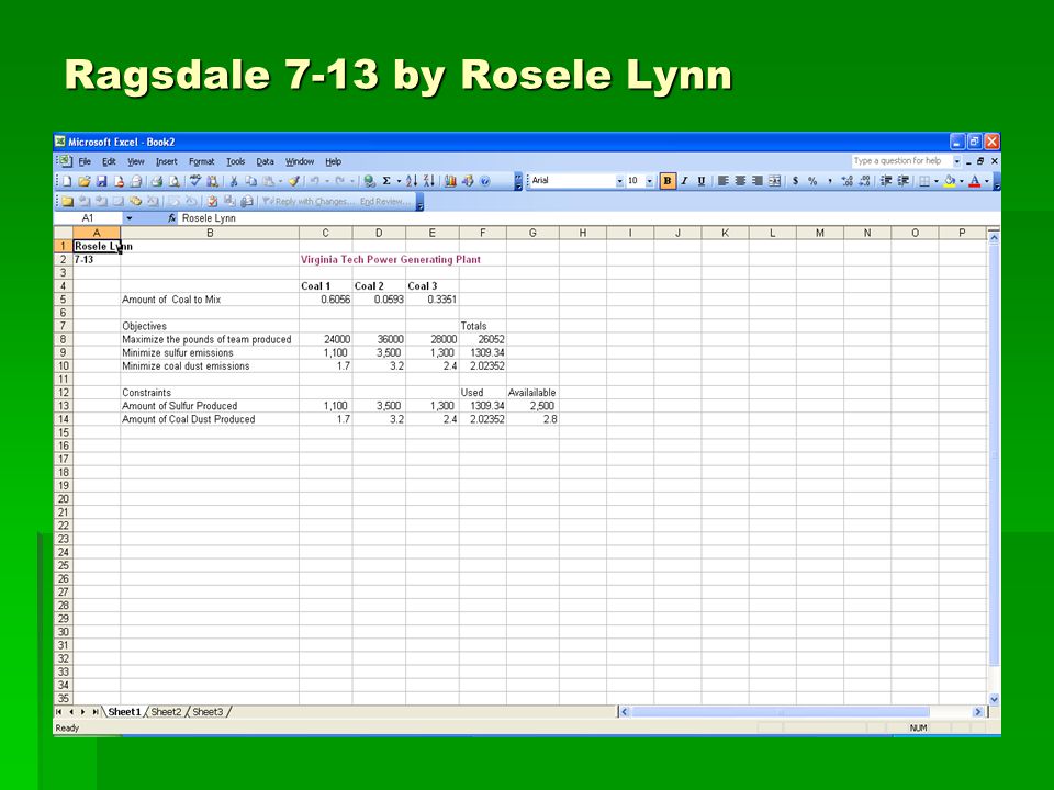
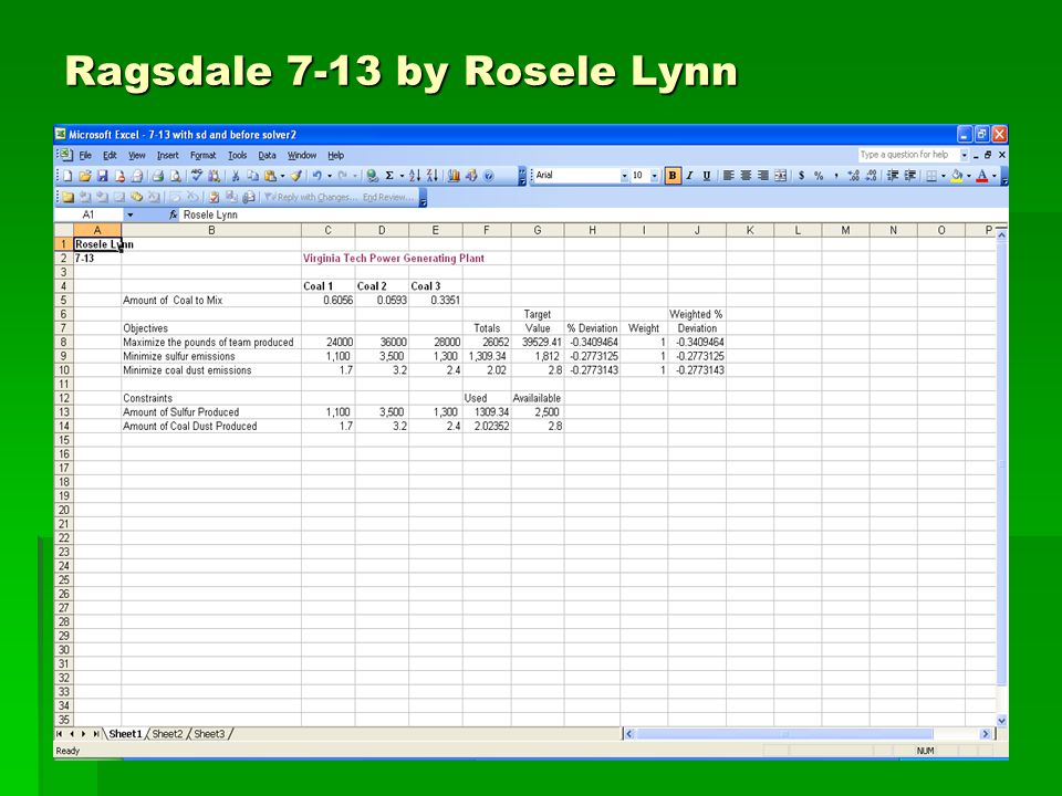
7. Ragsdale 7-13 by Rosele Lynn Problem: Which combination of three types of coal should be used in order to maintain the EPA’s requirements for sulfur and coal dust levels? Decision variables: Which combination of coal should be used? X1= coal type 1 X2= coal type 2 X3= coal type 3

8. Objective Functions: MAX: 24,000X1 + 36,000X2 + 28,000X3 } maximize steam produced MIN: 1,100X1 + 3,500X2 + 1,300X3 } minimize sulfur emissions MIN: 1.7X1 + 3.2X2 + 2.4X3 } minimize coal dust emissions Constraints: X1 + X2 > 0 } non-negativity constraint X1+ X2 + X3/3 < 2,500 } for each ton of coal burned less than 2,500 ppm sulfur X1+ X2 + X3/3 < 2.8 } for each ton of coal burned less than 2.8 kg coal dust Ragsdale 7-13 by Rosele Lynn

13. Ragsdale 7-19 by Jose F. Lopez (A & B) OBJECTIVES Maximize: 11X1 + 8X2 + 8.5X3 + 10X4 + 9X5 Average Yield on Funds Minimize: 8X1 + 1X2 + 7X3 + 6X4 + 2X5 Weighted Average Maturity Minimize: 5X1 + 2X2 + 1X3 + 5X4 + 3X5 Weighted Average Risk CONTRAINTS Subject to: 11X1 >= 0 10X4 >= 0 8X2 >= 0 9X5 >= 0 8.5X3 >= 0 11X1+8X2+8.5X3+10X4…. +9X5 = 1

14. Minimize: C16 By Changing: B5:B9, C16 Subject To: C14: D14 <= C16 B10 = 1 B5:B9 >= 0 Ragsdale 7-19 by Jose F. Lopez (A & B) Ragsdale 7-19 by Jose F. Lopez (A & B)

15. Minimize: C16 By Changing: B5:B9, C16 Subject To: C14: D14 <= C16 B10 = 1 B5:B9 >= 0 Ragsdale 7-19 by Jose F. Lopez (A & B)

16. Ragsdale 8-12 by Rosele Lynn Problem: How does Thom Pearman increase his life insurance coverage while keeping $6,000 in case of emergency? How does Pearman get the minimum amount of money to invest in order to have his after tax earnings cover his planned premium payments?

17. Ragsdale 8-12 by Rosele Lynn Ragsdale 8-12 by Rosele Lynn Spreadsheet before Solver

18. Ragsdale 8-12 by Rosele Lynn Ragsdale 8-12 by Rosele Lynn Solve for Annual Return

19. Ragsdale 8-12 by Rosele Lynn Ragsdale 8-12 by Rosele Lynn Minimum Investment with 15% Annual Rate

20. b. Solver tells us that this is a non linear model. Ragsdale 8-12 by Rosele Lynn

21. Ragsdale 8-22 by Deyanira Pena X1= location of new plant with respect to the x-axis Y1=location of new plant with respect to the y-axis Min:  (9-x1)^2 + (45-y1)^2) +  (2-x1)^2 + (28-y1)^2 +  (51-x1)^2 + (36-y1)^2 +  (19-X1)^2 + (4-Y1)^2 Subject to:  (9-x1)^2 + (45-y1)^2 } Dalton distance constraint  (9-x1)^2 + (45-y1)^2 } Dalton distance constraint  (2-x1)^2 + (28-y1)^2 }Rome distance constraint  (51-x1)^2 + (36-y1)^2 }Canton distance constraint  (19-X1)^2 + (4-Y1)^2}Kennesaw distance constraint  (19-X1)^2 + (4-Y1)^2}Kennesaw distance constraint

22. Minimize: C16 By Changing: B5:B9, C16 Subject To: C14: D14 <= C16 B10 = 1 B5:B9 >= 0 Ragsdale 8-22 by Deyanira Pena

23. Rugger Corporation Coordinates xyDistanceMaximum Plant12.4103529.69963 to Plant to PlantAllowed Dalton94313.73063088130 Rome22810.5481773875 Canton513639.1005889790 Kennesaw19426.531013480 Total89.91041063

24. Dielman 6-2 Dave Neal RESEARCH AND DEVELOPMENT A company is interested in the relationship between profit (PROFIT) on a number of projects and 2 explanatory variables. These variables are the expenditure on research and development (RD) and a measure of risk assigned at the outset of the project (RISK). PROFIT is measured in thousands of dollars and RD is measured in hundreds of dollars.

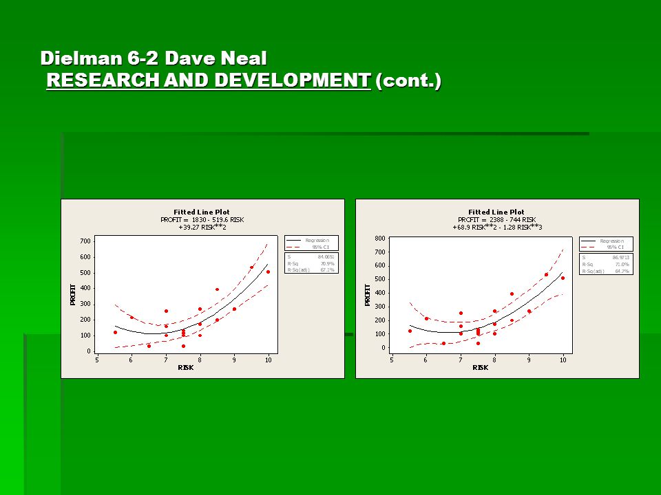
25. Dielman 6-2 Dave Neal RESEARCH AND DEVELOPMENT (cont.) 1.Using any of the given outputs, does the linearity assumption appear to be violated? Justify your answer.  PROFIT vs. RD appears to be linear. R 2 is 95.6%.  PROFIT vs. RD and RISK appears to be linear. R 2 is 99.2%.  PROFIT vs. RISK appears to violate the linearity assumption. R 2 is only 50.6%. 2.If you answered yes, state how the violation might be corrected.  PROFIT vs. RISK can be corrected by trying a quadratic and cubic polynomial regression analysis to see if the R 2 value is improved. 3.Then try your correction using a computer regression routine.  See the attached quadratic and cubic polynomial regression analysis data and plots. 4.Does your model appear to be an improvement over the original model? Justify your answer.  Yes, the quadratic and cubic polynomial regression analysis appears to be an improvement over the original model. R 2 improved from 50.6% to 71.0% within a 95% Confidence Interval.

26. Dielman 6-2 Dave Neal RESEARCH AND DEVELOPMENT (cont.) Regression Analysis: PROFIT versus RD The regression equation is PROFIT = - 295 + 5.21 RD Predictor Coef SE Coef T P Constant -294.84 28.05 -10.51 0.000 RD 5.2079 0.2808 18.54 0.000 S = 31.8337 R-Sq = 95.6% R-Sq(adj) = 95.3% Analysis of Variance Source DF SS MS F P Regression 1 348510 348510 343.91 0.000 Residual Error 16 16214 1013 Total 17 364724 ____________________________________________________________ Regression Analysis: PROFIT versus RISK The regression equation is PROFIT = - 490 + 90.5 RISK Predictor Coef SE Coef T P Constant -489.5 173.6 -2.82 0.012 RISK 90.45 22.33 4.05 0.001 S = 106.087 R-Sq = 50.6% R-Sq(adj) = 47.5% Analysis of Variance Source DF SS MS F P Regression 1 184652 184652 16.41 0.001 Residual Error 16 180072 11255 Total 17 364724

27. Dielman 6-2 Dave Neal RESEARCH AND DEVELOPMENT (cont.) Regression Analysis: PROFIT versus RD, RISK The regression equation is PROFIT = - 453 + 4.51 RD + 29.3 RISK Predictor Coef SE Coef T P Constant -453.18 23.51 -19.28 0.000 RD 4.5100 0.1538 29.33 0.000 RISK 29.309 3.669 7.99 0.000 S = 14.3420 R-Sq = 99.2% R-Sq(adj) = 99.0% Analysis of Variance Source DF SS MS F P Regression 2 361639 180820 879.08 0.000 Residual Error 15 3085 206 Total 17 364724 Source DF Seq SS RD 1 348510 RISK 1 13129 Unusual Observations Obs RD PROFIT Fit SE Fit Residual St Resid 9 152 536.00 508.94 7.98 27.06 2.27R 9 152 536.00 508.94 7.98 27.06 2.27R R denotes an observation with a large standardized residual.

28. Dielman 6-2 Dave Neal RESEARCH AND DEVELOPMENT (cont.)

30. Dielman 7-2 Thamer AbuDiak Graduation Rate  Variables:  y: Percentage of students who earned a bachelor degree in 4 years (GRADRATE4)  x 1 : Admission Rate expressed as a percentage (ADMINRATE)  x 2 : indicator variable coded as 1 for private and 0 for public school.  The regression equation is:  y = 0.589 - 0.350 x 1 + 0.282 x 2

31. Dielman 7-2 Thamer AbuDiak Graduation Rate a.F-test: i.F = (SSE R – SSE F )/(K-L)MSE F = (7.1215- 3.75) / (2*.0195) = 86.44 ii.Decision rule: i.H0 if F > 3.49 ii.Do not reject H0 if F <= 3.49 iii.Since 86 > 3.49, the null hypotheses is rejected. b.There are difference in the graduation rate between public and private schools.

32. Dielman 7-2 Thamer AbuDiak Graduation Rate c.Difference in graduation rates between public and private schools. Public school: y = 0.636 - 0.421 x 1Public school: y = 0.636 - 0.421 x 1 Private school y = 0.852 - 0.305 x 1Private school y = 0.852 - 0.305 x 1 Private schools have a higher graduation rate than public schools.Private schools have a higher graduation rate than public schools.

33. Dielman 7-2 Thamer AbuDiak Graduation Rate Sample graduation rate prediction d.

34. Dielman 7-2 Thamer AbuDiak Graduation Rate Regression without counting x2 as a factor Regression with counting x2 as a factor

35. S 11.1 10.8 11.0 R-Sq 99.88 99.88 99.87 R-Sq(adj) 99.86 99.87 99.86 Mallows C-p 5.0 3.0 2.6 StepConstant151.72251.17359.43 PaperT-valueP-value0.957.900.000.948.690.000.958.620.00 MachineT-valueP-value2.475.310.002.5111.010.002.3911.360.00 OverheadT-valueP-value0.050.090.927 LaborT-valueP-value-0.051-1.260.223-0.051-1.290.210 Dielman 8-1 Reynald Benoit Backward elimination. Alpha-to-Remove: 0.1 Response is COST on 4 predictors, with N = 27

36. Dielman 8-1 Reynald Benoit -cont  A) What is the equation?  COST = 59.43 + 0.95PAPER + 2.39MACHINE  B) What is the R2?  99.87%  C) What is the Adjusted R2?  99.86%  D) What is the standard error?  11.0  E) What variables were omitted? Are they related to cost?  Overhead and Labor. They are related to cost but paper and machine explains 99% of the variation in cost.