1. Introduction to R Graphics
Delia Voronca
2013

2. Objectives
Create basic graphical displays such as scatter plots, boxplots, histograms, interaction plots and 3-D plots
Change plot symbols, add an arbitrary straight line, add points or lines, add an OLS line fit to points, add a normal density curve to a histogram
Add titles, footnotes, mathematical symbols, arrows and shapes
Add a legend
Change size of the graph, point, text, margins, put multiple plots per page
Changes axis, line styles, add colors
Save graphs

3. Useful Plots Scatterplot Multiple y values plot(x, y) plot(x, y1)
points(x, y2)
points(x, y3)
...
Use pch=“d” and
pch=“h” to change
the plotting symbols

4. Useful Plots
Barpot
barplot(table(x1, x2), legend=c(“x1.grp1", “x1.grp2"), xlab="X2“, beside=TRUE) Or
library(lattice)
barchart(table(x1,x2,x3))

5. Useful Plots Histogram Stem-and-leaf Plot hist(x) stem(x)
The decimal point is at the |
1 |
2 |
3 | 000
4 |
5 |
6 | 0
7 |
8 | 0

6. Useful Plots Side-by-side boxplots Boxplots and Violin Plots
boxplot(x)
horizontal = TRUE
library(vioplot)
vioplot(x1, x2, x3)
Side-by-side boxplots
boxplot(y~x) Or
library(lattice)
bwplot(y~x)

7. Useful Plots Quantile-quantile plots qqnorm(x) qqline(x)
Quantile – Quantile-Quantile plot
qqplot(x, y)

8. Useful Plots Interaction plot
Display means by 2 variables (in a two-way analysis of variance)
interaction.plot(x1, x2, y)
fun (option to change default statistic which is the mean)

9. Useful Plots Empirical probability density plot
Density plots are non-parametric estimates of the empirical probability density function
#univariate density
plot(density(x))
One could compare groups
by looking at kernel density
plots

10. Useful Plots 3 – D plots persp(x, y, z) contour(x, y, z)
Image(x, y, z) OR
library(scatterplot3d)
scatterplot3d(x, y, z)
The values for x and y must be in ascending order

11. Adding Elements Add an arbitrary straight line: Plot symbols
plot(x, y)
abline(intercept, slope)
Plot symbols
plot(x, y, pch=pchval)
PCH symbols used in R
“col=“ and “bg=” are also specified
PCH can also be in characters such as
“A”, “a”, “%” etc.

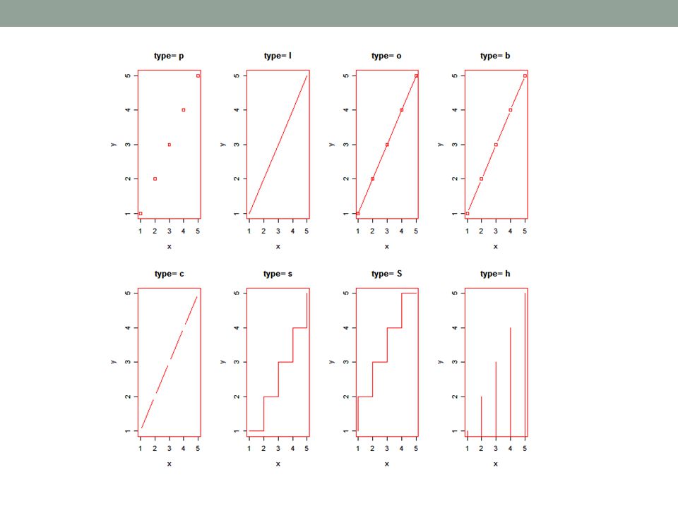
12. Adding Elements Adding Points or Lines to an Existing Graphic
plot(x, y)
points(x, y)
lines(x, y, type=“type”)
type =
p points
l lines
o overplotted points and lines
b, c points (empty if "c") joined by lines
s, S stair steps
h histogram-like vertical lines
n does not produce any points or lines
OLS line fit to the points
abline(lm(y~x))

14. Adding Elements Add a Normal Curve
h<-hist(x, breaks=10, col="red", xlab=“Xlab",
main="Histogram with Normal Curve")
xfit<-seq(min(x),max(x),length=40)
yfit<-dnorm(xfit,mean=mean(x),sd=sd(x))
yfit <- yfit*diff(h$mids[1:2])*length(x)
lines(xfit, yfit, col="blue", lwd=2)

15. Adding Elements Titles Mathematical Symbols Arrows and Shapes
title(main=“main” , sub = “sub”, xlab=“xlab”, ylab=“ylab”)
Mathematical Symbols
plot(x, y)
expr = expression(paste(mathexpression)))
title(xlab=c(expr))
Arrows and Shapes
arrows(x, y)
rect(xleft, ybottom, xright, ytop)
polygon(x, y)
library(plotrix)
draw.circle(x, y, r)

16. Adding Elements Legend plot(x, y)
legend(xval, yval, legend = c(“Grp1”, “Grp2”), lty=1:2, col=3:4, bty=“box type”)
Add a legend at the location at (xval, yval)
A vector of legend labels, line types,
and colors can be specified
using legend, lty and col options.
bty =“o” or “n”

17. Options and Parameters
Graph Size
pdf(“filename.pdf”, width = Xin, height = Yin)
Point and text size
plot(x, y, cex = cexval)
cex number indicating the amount by which plotting text and symbols should be scaled relative to the default. 1=default, 1.5 is 50% larger, 0.5 is 50% smaller, etc.
cex.axis magnification of axis annotation relative to cex
cex.lab magnification of x and y labels relative to cex
cex.main magnification of titles relative to cex
cex.sub magnification of subtitles relative to cex
Box around plots
plot(x, y, bty = btyval)

18. Options and Parameters
Size of margins
par(mar=c(bot, left, top, right))
Save graphical settings
par() #view currents settings
opar <- par() #make a copy of current settings
par(opar) #restore original settings
Multiple plots per page
par(mfrow=c(a, b)) #a rows and b columns
par(mfcol=c(a,b))

19. Options and Parameters
Axis Range and Style
plot(x, y, xlim = c(minx, maxx), ylim = c (miny, maxy), xaxs=“i”, yaxs=“i”)
The xaxs and yaxs control whether the tick marks extend beyond the limits of the plotted observations (default) or are constrained to be internal (“i”)
See also:
axis()
mtext()
Omit axis
plot(x, y, xaxt = “n”, yaxy=“n”)

20. Options and Parameters
Axis labels, values, and tick marks
plot(x, y, lab=c(x, y, len), #number of tick marks
las=lasval, #orientation of tick marks
tck = tckval, #length of tick marks
xaxp = c(x1, x2, n), #coordinates of the extreme tick marks
yaxp = c(x1, x2, n),
xlab = “X axis label”, ylab=“Y axis label”)
las = 0 labels are parallel to axis
las=2 labels are perpendicular to axis
tck = 0 suppresses the tick mark

21. Options and Parameters
Line styles, line width and colors
plot(….)
lines(x, y, lty=ltyval, lwd = lwdval,
col=colval)
col Default plotting color. Some functions (e.g. lines) accept a vector of values that are recycled.
col.axis color for axis annotation
col.lab color for x and y labels
col.main color for titles
col.sub color for subtitles
fg plot foreground color (axes, boxes - also sets col= to same)
bg plot background color

22. Options and Parameters
More on how to change colors
You can specify colors in R by index, name, hexadecimal, or RGB.
For example col=1, col="white", and col="#FFFFFF" are equivalent.
colors() #list of color names

23. Options and Parameters
Fonts
font Integer specifying font to use for text.
1=plain, 2=bold, 3=italic, 4=bold italic, 5=symbol
font.axis font for axis annotation
font.lab font for x and y labels
font.main font for titles
font.sub font for subtitles
ps font point size (roughly 1/72 inch)
text size=ps*cex
family font family for drawing text. Standard values are "serif", "sans", "mono", "symbol".

24. Saving Graphs pdf(“file.pdf”) plot(….) dev.off() jpeg(“file.jpeg”)
win.metafile(file.wmf)
Similar code for BMP, TIFF, PNG, POSTSCRIPT
PNG is usually recommended
The dev.off() function is used to close the graphical device

25. Go Over R Code

26. In Class Activity Any ideas on how to reproduce this graph?
What are some things
you need to know?
Data and ICC formula
Add a title
Change axis labels
Change tick marks
Change color
Add legend
Change font and size
*Use a for loop

27. In Class Activity
Let’s go over the code
Questions
Homework

28. References
SAS and R – data Management, Statistical Analysis, and Graphics, Ken Kleinman and Nicholas J. Horton
Quick – R :
R help