1. Graphs (Part II) Shannon Quinn (with thanks to William Cohen and Aapo Kyrola of CMU, and J. Leskovec, A. Rajaraman, and J. Ullman of Stanford University)

2. Parallel Graph Computation Distributed computation and/or multicore parallelism – Sometimes confusing. We will talk mostly about distributed computation. Are classic graph algorithms parallelizable? What about distributed? – Depth-first search? – Breadth-first search? – Priority-queue based traversals (Djikstra’s, Prim’s algorithms)

3. MapReduce for Graphs Graph computation almost always iterative MapReduce ends up shipping the whole graph on each iteration over the network (map- >reduce->map->reduce->...) – Mappers and reducers are stateless

4. Iterative Computation is Difficult System is not optimized for iteration: Data CPU 1 CPU 2 CPU 3 Data CPU 1 CPU 2 CPU 3 Data CPU 1 CPU 2 CPU 3 Iterations Disk Penalty Startup Penalty

5. MapReduce and Partitioning Map-Reduce splits the keys randomly between mappers/reducers But on natural graphs, high-degree vertices (keys) may have million-times more edges than the average  Extremely uneven distribution  Time of iteration = time of slowest job.

6. Curse of the Slow Job Data CPU 1 CPU 2 CPU 3 CPU 1 CPU 2 CPU 3 Data CPU 1 CPU 2 CPU 3 Iterations Barrier Data Barrier http://www.www2011india.com/proceeding/proceedings/p607.pdf

7. Map-Reduce is Bulk-Synchronous Parallel Bulk-Synchronous Parallel = BSP (Valiant, 80s) – Each iteration sees only the values of previous iteration. – In linear systems literature: Jacobi iterations Pros: – Simple to program – Maximum parallelism – Simple fault-tolerance Cons: – Slower convergence – Iteration time = time taken by the slowest node

8. Triangle Counting in Twitter Graph 40M Users 1.2B Edges Total: 34.8 Billion Triangles Hadoop results from [Suri & Vassilvitskii '11] 1536 Machines 423 Minutes 64 Machines, 1024 Cores 1.5 Minutes

9. PageRank 40M Webpages, 1.4 Billion Links (100 iterations) 5.5 hrs 1 hr 8 min Hadoop results from [Kang et al. '11] Twister (in-memory MapReduce) [Ekanayake et al. ‘10]

10. Graph algorithms PageRank implementations – in memory – streaming, node list in memory – streaming, no memory – map-reduce A little like Naïve Bayes variants – data in memory – word counts in memory – stream-and-sort – map-reduce

11. Google ’ s PageRank web site xxx web site yyyy web site a b c d e f g web site pdq pdq.. web site yyyy web site a b c d e f g web site xxx Inlinks are “ good ” (recommendations) Inlinks from a “ good ” site are better than inlinks from a “ bad ” site but inlinks from sites with many outlinks are not as “ good ”... “ Good ” and “ bad ” are relative. web site xxx

12. Google ’ s PageRank web site xxx web site yyyy web site a b c d e f g web site pdq pdq.. web site yyyy web site a b c d e f g web site xxx Imagine a “ pagehopper ” that always either follows a random link, or jumps to random page

13. Google ’ s PageRank (Brin & Page, http://www-db.stanford.edu/~backrub/google.html) web site xxx web site yyyy web site a b c d e f g web site pdq pdq.. web site yyyy web site a b c d e f g web site xxx Imagine a “ pagehopper ” that always either follows a random link, or jumps to random page PageRank ranks pages by the amount of time the pagehopper spends on a page: or, if there were many pagehoppers, PageRank is the expected “ crowd size ”

14. Random Walks avoids messy “dead ends”….

15. Random Walks: PageRank

17. Graph = Matrix Vector = Node  Weight H ABCDEFGHIJ A_111 B1_1 C11_ D_11 E1_1 F111_ G_11 H_11 I11_1 J111_ A B C F D E G I J A A3 B2 C3 D E F G H I J M M v

18. PageRank in Memory Let u = (1/N, …, 1/N) – dimension = #nodes N Let A = adjacency matrix: [a ij =1  i links to j] Let W = [w ij = a ij /outdegree(i)] – w ij is probability of jump from i to j Let v 0 = (1,1,….,1) – or anything else you want Repeat until converged: – Let v t+1 = cu + (1-c)Wv t c is probability of jumping “anywhere randomly”

19. Streaming PageRank Assume we can store v but not W in memory Repeat until converged: – Let v t+1 = cu + (1-c)Wv t Store A as a row matrix: each line is – i j i,1,…,j i,d [the neighbors of i] Store v’ and v in memory: v’ starts out as cu For each line “i j i,1,…,j i,d “ – For each j in j i,1,…,j i,d v’[j] += (1-c)v[i]/d Everything needed for update is right there in row….

20. Streaming PageRank: with some long rows Repeat until converged: – Let v t+1 = cu + (1-c)Wv t Store A as a list of edges: each line is: “i d(i) j” Store v’ and v in memory: v’ starts out as cu For each line “i d j“ v’[j] += (1-c)v[i]/d We need to get the degree of i and store it locally

21. Streaming PageRank: preprocessing Original encoding is edges (i,j) Mapper replaces i,j with i,1 Reducer is a SumReducer Result is pairs (i,d(i)) Then: join this back with edges (i,j) For each i,j pair: – send j as a message to node i in the degree table messages always sorted after non-messages – the reducer for the degree table sees i,d(i) first then j1, j2, …. can output the key,value pairs with key=i, value=d(i), j

22. Preprocessing Control Flow: 1 IJ i1j1,1 i1j1,2 …… i1j1,k1 i2j2,1 …… i3j3,1 …… I i11 1 …… 1 i21 …… i31 …… I i11 1 …… 1 i21 …… i31 …… Id(i) i1d(i1)..… i2d(i2) …… i3d)i3) …… MAP SORT REDUCE Summing values

23. Preprocessing Control Flow: 2 IJ i1j1,1 i1j1,2 …… i2j2,1 …… I i1d(i1) i1~j1,1 i1~j1,2..… i2d(i2) i2~j2,1 i2~j2,2 …… I i1d(i1)j1,1 i1d(i1)j1,2 ……… i1d(i1)j1,n1 i2d(i2)j2,1 ……… i3d(i3)j3,1 ……… Id(i) i1d(i1)..… i2d(i2) …… MAP SORT REDUCE IJ i1~j1,1 i1~j1,2 …… i2~j2,1 …… Id(i) i1d(i1)..… i2d(i2) …… copy or convert to messagesjoin degree with edges

24. Control Flow: Streaming PR IJ i1j1,1 i1j1,2 …… i2j2,1 …… Id/v i1d(i1),v(i1) i1~j1,1 i1~j1,2..… i2d(i2),v(i2) i2~j2,1 i2~j2,2 …… todelta i1c j1,1(1-c)v(i1)/d(i1) …… j1,n1i i2c j2,1… …… i3c Id/v i1d(i1),v(i1) i2d(i2),v(i2) …… MAP SORT REDUCE MAP SORT Idelta i1c (1-c)v(…)…. i1(1-c)…..… i2c (1-c)… i2…. …… copy or convert to messages send “pageRank updates ” to outlinks

25. Control Flow: Streaming PR todelta i1c j1,1(1-c)v(i1)/d(i1) …… j1,n1i i2c j2,1… …… i3c REDUCE MAP SORT Idelta i1c (1-c)v(…)…. i1(1-c)…..… i2c (1-c)… i2…. …… REDUCE Iv’ i1~v’(i1) i2~v’(i2) …… Summing values Id/v i1d(i1),v(i1) i2d(i2),v(i2) …… MAP SORT REDUCE Replace v with v’ Id/v i1d(i1),v’(i1) i2d(i2),v’(i2) ……

26. Control Flow: Streaming PR IJ i1j1,1 i1j1,2 …… i2j2,1 …… Id/v i1d(i1),v(i1) i2d(i2),v(i2) …… MAP copy or convert to messages and back around for next iteration….

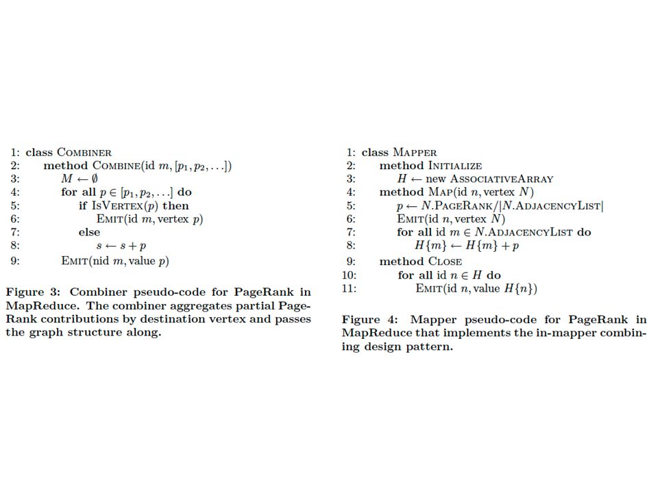
27. PageRank in MapReduce

28. More on graph algorithms PageRank is a one simple example of a graph algorithm – but an important one – personalized PageRank (aka “random walk with restart”) is an important operation in machine learning/data analysis settings PageRank is typical in some ways – Trivial when graph fits in memory – Easy when node weights fit in memory – More complex to do with constant memory – A major expense is scanning through the graph many times … same as with SGD/Logistic regression disk-based streaming is much more expensive than memory-based approaches Locality of access is very important! gains if you can pre-cluster the graph even approximately avoid sending messages across the network – keep them local

29. Machine Learning in Graphs - 2010

30. Some ideas Combiners are helpful – Store outgoing incrementVBy messages and aggregate them – This is great for high indegree pages Hadoop’s combiners are suboptimal – Messages get emitted before being combined – Hadoop makes weak guarantees about combiner usage

31. This slide again!

34. Some ideas Most hyperlinks are within a domain – If we keep domains on the same machine this will mean more messages are local – To do this, build a custom partitioner that knows about the domain of each nodeId and keeps nodes on the same domain together – Assign node id’s so that nodes in the same domain are together – partition node ids by range – Change Hadoop’s Partitioner for this

35. Some ideas Repeatedly shuffling the graph is expensive – We should separate the messages about the graph structure (fixed over time) from messages about pageRank weights (variable) – compute and distribute the edges once – read them in incrementally in the reducer not easy to do in Hadoop! – call this the “Schimmy” pattern

36. Schimmy Relies on fact that keys are sorted, and sorts the graph input the same way…..

37. Schimmy

38. Results

39. More details at… Overlapping Community Detection at Scale: A Nonnegative Matrix Factorization Approach by J. Yang, J. Leskovec. ACM International Conference on Web Search and Data Mining (WSDM), 2013. Overlapping Community Detection at Scale: A Nonnegative Matrix Factorization Approach Detecting Cohesive and 2-mode Communities in Directed and Undirected Networks by J. Yang, J. McAuley, J. Leskovec. ACM International Conference on Web Search and Data Mining (WSDM), 2014. Detecting Cohesive and 2-mode Communities in Directed and Undirected Networks Community Detection in Networks with Node Attributes by J. Yang, J. McAuley, J. Leskovec. IEEE International Conference On Data Mining (ICDM), 2013. Community Detection in Networks with Node Attributes J. Leskovec, A. Rajaraman, J. Ullman: Mining of Massive Datasets, http://www.mmds.org 39

40. Resources Stanford SNAP datasets: – http://snap.stanford.edu/data/index.html http://snap.stanford.edu/data/index.html ClueWeb (CMU): – http://lemurproject.org/clueweb09/ http://lemurproject.org/clueweb09/ Univ. of Milan’s repository: – http://law.di.unimi.it/datasets.php http://law.di.unimi.it/datasets.php