Download presentation
Presentation is loading. Please wait.

1
CBM Calorimeter System CBM collaboration meeting, October 2008 I.Korolko(ITEP, Moscow)
")
2
Outline ■ Particle identification in ECAL (longitudinal segmentation) Y.Kharlov, A.Artamonov ■ Reconstruction in the CBM ECAL M.Prokudin ■ Optimization of the CBM ECAL I.Korolko
 Y.Kharlov, A.Artamonov ■ Reconstruction in the CBM ECAL M.Prokudin ■ Optimization of the CBM ECAL I.Korolko")
3
PID in CBM In CBM, the particle identification (PID) is realized in TOF, TRD, RICH and ECAL The main object of ECAL PID is to discriminate photons and e+- from other particles The ECAL PID is based mainly on an investigation of transverse shower shape analysis A subject of this study is to perform the ECAL PID by using just longitudinal shower shape analysis The most simple case has been studied when ECAL module consists of 2 longitudinal segments This case is very close to the current design of ECAL, since it consists of preshower and ECAL modules Method used is to analyse 2D plot, namely an energy deposition in the 1 st segment of ECAL module versus an energy deposition in the whole ECAL module
 is realized in TOF, TRD, RICH and ECAL The main object of ECAL PID is to discriminate photons and e+- from other particles The ECAL PID is based mainly on an investigation of transverse shower shape analysis A subject of this study is to perform the ECAL PID by using just longitudinal shower shape analysis The most simple case has been studied when ECAL module consists of 2 longitudinal segments This case is very close to the current design of ECAL, since it consists of preshower and ECAL modules Method used is to analyse 2D plot, namely an energy deposition in the 1 st segment of ECAL module versus an energy deposition in the whole ECAL module")
4
Framework – cbmroot as a new detector module segcal 1 ECAL module with 160 layers (Pb 0.7 mm + Sci 1.0 mm) 20 longitudinal segments, each one consists of 8 layers Effective radiation length of the ECAL module: 1.335 cm Total radiation length of the ECAL module: 20.4 X0 A single primary particle (photon, muon, pion, kaon, proton, neutron, antineutron and Lambda(1115)) with energies 1, 2, 3,..., 23, 24, 25 GeV Simulation model
 20 longitudinal segments, each one consists of 8 layers Effective radiation length of the ECAL module: cm Total radiation length of the ECAL module: 20.4 X0 A single primary particle (photon, muon, pion, kaon, proton, neutron, antineutron and Lambda(1115)) with energies 1, 2, 3,..., 23, 24, 25 GeV Simulation model")
5
Various combinations of segment thickness: 1 X0 (in 1 st segment) + 19 X0 (in 2 nd segment) 2 X0 (in 1 st segment) + 18 X0 (in 2 nd segment) 3 X0 (in 1 st segment) + 17 X0 (in 2 nd segment) 4 X0 (in 1 st segment) + 16 X0 (in 2 nd segment) 5 X0 (in 1 st segment) + 15 X0 (in 2 nd segment) 6 X0 (in 1 st segment) + 14 X0 (in 2 nd segment) 7 X0 (in 1 st segment) + 13 X0 (in 2 nd segment) 8 X0 (in 1 st segment) + 12 X0 (in 2 nd segment) 9 X0 (in 1 st segment) + 11 X0 (in 2 nd segment) 10 X0 (in 1 st segment) + 10 X0 (in 2 nd segment) 11 X0 (in 1 st segment) + 9 X0 (in 2 nd segment) 12 X0 (in 1 st segment) + 8 X0 (in 2 nd segment) 13 X0 (in 1 st segment) + 7 X0 (in 2 nd segment) 14 X0 (in 1 st segment) + 6 X0 (in 2 nd segment) 15 X0 (in 1 st segment) + 5 X0 (in 2 nd segment) 16 X0 (in 1 st segment) + 4 X0 (in 2 nd segment) 17 X0 (in 1 st segment) + 3 X0 (in 2 nd segment) 18 X0 (in 1 st segment) + 2 X0 (in 2 nd segment) 19 X0 (in 1 st segment) + 1 X0 (in 2 nd segment) Particle identification is based on relation between the total energy and the energy in the first segment: E 1 vs E tot
 + 19 X0 (in 2 nd segment) 2 X0 (in 1 st segment) + 18 X0 (in 2 nd segment) 3 X0 (in 1 st segment) + 17 X0 (in 2 nd segment) 4 X0 (in 1 st segment) + 16 X0 (in 2 nd segment) 5 X0 (in 1 st segment) + 15 X0 (in 2 nd segment) 6 X0 (in 1 st segment) + 14 X0 (in 2 nd segment) 7 X0 (in 1 st segment) + 13 X0 (in 2 nd segment) 8 X0 (in 1 st segment) + 12 X0 (in 2 nd segment) 9 X0 (in 1 st segment) + 11 X0 (in 2 nd segment) 10 X0 (in 1 st segment) + 10 X0 (in 2 nd segment) 11 X0 (in 1 st segment) + 9 X0 (in 2 nd segment) 12 X0 (in 1 st segment) + 8 X0 (in 2 nd segment) 13 X0 (in 1 st segment) + 7 X0 (in 2 nd segment) 14 X0 (in 1 st segment) + 6 X0 (in 2 nd segment) 15 X0 (in 1 st segment) + 5 X0 (in 2 nd segment) 16 X0 (in 1 st segment) + 4 X0 (in 2 nd segment) 17 X0 (in 1 st segment) + 3 X0 (in 2 nd segment) 18 X0 (in 1 st segment) + 2 X0 (in 2 nd segment) 19 X0 (in 1 st segment) + 1 X0 (in 2 nd segment) Particle identification is based on relation between the total energy and the energy in the first segment: E 1 vs E tot")
6
The energy deposition in the whole module caused by 2 GeV photon and 1,2,3,4 GeV/c neutron Neutron contamination to photon spectrum: 1D case

7
The energy deposition in the 1st segment versus the full energy deposition. Black points correspond to 2 GeV photons, red points correspond to 1 GeV/c neutrons. Segmentation: 10 X0 (1st segment) + 10 X0 (2nd segment) Neutron contamination to photon spectrum 2D case
 + 10 X0 (2nd segment) Neutron contamination to photon spectrum 2D case.")
8
The energy deposition in the 1st segment versus the energy deposition in the whole module. The same plot but with one additional population originated from 2 GeV/c neutrons (blue points) Neutron contamination to photon spectrum 2D case
 Neutron contamination to photon spectrum 2D case.")
9
The energy deposition in the 1st segment versus the energy deposition in the whole module. The same plot but with one additional population originated from 3 GeV/c neutrons (green points) Neutron contamination to photon spectrum 2D case
 Neutron contamination to photon spectrum 2D case.")
10
The energy deposition in the 1st segment versus the energy deposition in the whole module. The same plot but with one additional population originated from 4 GeV/c neutrons (magenta points) Neutron contamination to photon spectrum 2D case
 Neutron contamination to photon spectrum 2D case.")
11
Probabilities for neutron to fake 2 GeV photon. This plot corresponds to the following segment structure: 10X0+10X0

12
Probabilities for neutron to fake 1, 2, 3, 4, 5, 6, 7, 8, 9, 10, 11,..., 23, 24 and 25 GeV photons. Segment structure: 10X0+10X0

13
Probabilities for neutron to fake 2 GeV photon in module with 2 segments 10X0+10X0 (red curve) and the whole module (black curve)
 and the whole module (black curve)")
14
Probabilities for neutron to fake 10 GeV photon in module with 2 segments 10X0+10X0 (red curve) and the whole module (black curve)
 and the whole module (black curve)")
15
Definition of convolution integral

16
Probabilities for neutron with any momentum to fake photon with a given energy in module with 2 segments 10X0+10X0 (red curve) and the whole module (black curve) Integral contamination of photon spectrum by neutrons
 and the whole module (black curve) Integral contamination of photon spectrum by neutrons")
17
Ratio of probabilities for neutron with any momentum to fake photon with a given energy 1-segmented modules vs 2-segmented one

18
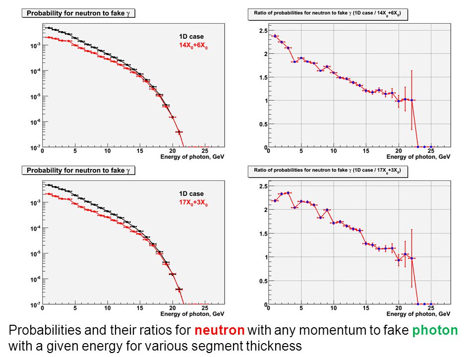
Probabilities and their ratios for neutron with any momentum to fake photon with a given energy for various segment thickness

20
The 1 st practical realization of the well known procedure for performing the ECAL PID in the 1D case (whole ECAL module) and the 2D case (ECAL module with 2 segments) were done The probabilities for hadrons and muons of various momenta P to fake a photon of various energies E were obtained. For example, in the segment structure 14X0+6X0, 5 GeV photon can be faked by 5.3e-03 of 6 GeV/c neutrons, by 2.9e-02 of 6 GeV/c K0L, by 4.8e-02 of 6 GeV/c antineutrons, by 5.1e-03 of 6 GeV/c Lambda(1115), by 4.7e-02 of 6 GeV/c pi-, by 3.4e-02 of 6 GeV/c pi+, by 5.4e-03 of 6 GeV/c protons, by 6.0e-05 of 7 GeV/c muons The probabilities for hadrons of ANY momenta P (integrated over momenta of the hadrons) to fake a photon of various energies E were obtained. For example, in the segment structure 14X 0 +6X 0, 5 GeV photon can be faked by 9.1 10 -4 of neutrons, 1.7 10 -4 of K 0 L, 3.5 10 -6 of antineutrons, 1.5 10 -4 of Lambda(1115), 1.2 10 -3 of -, 9.8 10 -4 of +, 8.8 10 -4 of protons PID has been studied for 19 combinations of segment thickness. The most optimum segment combinations are 14X 0 +6X 0 and 15X 0 +5X 0. Conclusion
, by 4.7e-02 of 6 GeV/c pi-, by 3.4e-02 of 6 GeV/c pi+, by 5.4e-03 of 6 GeV/c protons, by 6.0e-05 of 7 GeV/c muons The probabilities for hadrons of ANY momenta P (integrated over momenta of the hadrons) to fake a photon of various energies E were obtained. For example, in the segment structure 14X 0 +6X 0, 5 GeV photon can be faked by 9.1 of neutrons, 1.7 of K 0 L, 3.5 of antineutrons, 1.5 of Lambda(1115), 1.2 of -, 9.8 of +, 8.8 of protons PID has been studied for 19 combinations of segment thickness. The most optimum segment combinations are 14X 0 +6X 0 and 15X 0 +5X 0. Conclusion.")
21
Outline Calorimeter software development –photon reconstruction cluster finder simple reconstruction –UrQMD events –matching –Calorimeter drawing tools Cluster fitting –requirements Conclusions Next steps

22
Photon reconstruction. Requirements Robust reconstruction of single photons Two close photons case: –robust reconstruction of parameters in case two separate maximums –separation one/two photons in case of one maximum Fast! (should be)
.")
23
Calorimeter drawing tools Photons –MC –Reconstructed * (Anti) neutrons Charged tracks –Reconstructed * –MC Secondary –Photons –Electrons
 neutrons Charged tracks –Reconstructed * –MC Secondary –Photons –Electrons")
24
Shower width Energy deposition in cluster cells are not independent –storing of RMS in shower library useless Analytical formula –with correlation ALICE –σ 2 =c 0 (E meas +c 1 ) no correlations! PHENIX –σ 2 =c 0 (E meas (1- E meas /E cluster ) (1+k sin 4 θE cluster )+c 1 ) correlations are in –Angle dependence shower library h4 h5
 (1+k sin 4 θE cluster )+c 1 ) correlations are in –Angle dependence shower library h4 h5.")
25
χ 2 distributions. Single photons 95% 1 GeV95% 4 GeV σ 2 =c 0 (E meas (1-E meas /E cluster )+c 1 ) c1=0.0005 95% 1 GeV95% 4 GeV σ 2 =c 0 (E meas +c 1 ) Shape of χ 2 for each energy looks Ok, but cut with 95% efficiency has different value! Need a different σ 2 formula!
+c 1 ) c1= % 1 GeV95% 4 GeV σ 2 =c 0 (E meas +c 1 ) Shape of χ 2 for each energy looks Ok, but cut with 95% efficiency has different value. Need a different σ 2 formula!.")
26
Rejection power. Inner region σ 2 =c 0 (E meas (1-E meas /E cluster )+c 1 )σ 2 =c 0 (E meas +c 1 )
+c 1 )σ 2 =c 0 (E meas +c 1 ).")
27
Rejection power. Outer region σ 2 =c 0 (E meas (1-E meas /E cluster )+c 1 )σ 2 =c 0 (E meas +c 1 ) Reconstruction in outer region is most sensible to σ 2 formula!
+c 1 )σ 2 =c 0 (E meas +c 1 ) Reconstruction in outer region is most sensible to σ 2 formula!.")
28
Goals of the optimization The main goal of the optimization is to fit in budget (which is not defined yet) ■ keeping possibility to reconstruct γ, π 0, η, … ■ keeping wide Θ acceptance ■ keeping electron identification ■ remove low populated cells (outer region) ■ remove hot cells (central region) Reduce calorimeter acceptance (24K channels)
 ■ keeping possibility to reconstruct γ, π 0, η, … ■ keeping wide Θ acceptance ■ keeping electron identification ■ remove low populated cells (outer region) ■ remove hot cells (central region) Reduce calorimeter acceptance (24K channels)")
29
Hot cells The amount of material between target and calorimeter is (most probably) underestimated
 underestimated")
30
Strategy of optimization Study efficiency of π 0 and η reconstruction normalized with number of ECAL channels What is the optimal shape ? What is the optimal acceptance ? Do we need two arms ? Do we need central region ?

31
Calorimeter shape Two rectangular arms are better

32
Do we need the central region ? Central region is rather useful (even taking into account high occupancy)
.")
33
Efficiency vs Θ Calculated for two arm calorimeter with ~14000 channels

34
Efficiency vs P t Calculated for two arm calorimeter with ~14000 channels

35
New calorimeter Main features ~14K channels Efficient γ, π 0, η reconstruction Electron identification Movable design (no central region)
")
Similar presentations


 CBM Collaboration meeting, October 2004.>")

