1. Bayesian Hypothesis Testing In Nested Models Harold Jeffreys Jeff Rouder

2. Bayesian Hypothesis Testing: Example  We prepare for you a series of 10 factual true/false questions of equal difficulty.  You answer 9 out of 10 questions correctly.  Have you been guessing?

3. Bayesian Hypothesis Testing: Example  The Bayesian hypothesis test starts by calculating, for each model, the (marginal) probability of the observed data.  The ratio of these quantities is called the Bayes factor:

4. Bayesian Hypothesis Testing: Example  BF 01 = p(D|H 0 ) / p(D|H 1 )  When BF 01 = 2, the data are twice as likely under H 0 as under H 1.  When, a priori, H 0 and H 1 are equally likely, this means that the posterior probability in favor of H 0 is 2/3.

5. Bayesian Hypothesis Testing: Example  The complication is that these so-called marginal probabilities are often difficult to compute.  For this simple model, everything can be done analytically…

6. Bayesian Hypothesis Testing: Example  BF 01 = p(D|H 0 ) / p(D|H 1 ) = 0.107  This means that the data are 1/ 0.107 = 9.3 times more likely under H 1, the “no-guessing” model.  The associated posterior probability for H 0 is about 0.10.  For more interesting models, things are never this straightforward!

7. Savage-Dickey  When the competing models are nested (i.e., one is a more complex version of the other), Savage and Dickey have shown that, in our example,

8. Savage-Dickey Height of prior distribution at point of interest Height of posterior distribution at point of interest

9. Height of prior = 1 Height of posterior = 0.107; Therefore, BF 01 = 0.107/1 = 0.107.

10. Advantages of Savage-Dickey  In order to obtain the Bayes factor you do not need to integrate out the model parameters, as you would do normally.  Instead, you only needs to work with the more complex model, and study the prior and posterior distributions only for the parameter that is subject to test.

11. Practical Problem  Dr. John proposes a Seasonal Memory Model (SMM), which quickly becomes popular.  Dr. Smith is skeptical, and wants to test the model.  The model predicts that the increase in recall performance due to the intake of glucose is more pronounced in summer than in winter.  Dr. Smith conducts the experiment…

12. Practical Problem  And finds the following results:  For these data, t = 0.79, p =.44.  Note that, if anything, the result goes in the direction opposite to that predicted by the model.

13. Practical Problem  Dr. Smith reports his results in a paper entitled “False Predictions from the SMM: The impact on glucose and the seasons on memory”, which he submits to the Journal of Experimental Psychology: Learning, Memory, and Seasons.  After some time, Dr. Smith receives three reviews, one signed by Dr. John, who invented the SMM. Part of this review reads:

14. Practical Problem “From a null result, we cannot conclude that no difference exists, merely that we cannot reject the null hypothesis. Although some have argued that with enough data we can argue for the null hypothesis, most agree that this is only a reasonable thing to do in the face of a sizeable amount of data [which] has been collected over many experiments that control for all concerns. These conditions are not met here. Thus, the empirical contribution here does not enable readers to conclude very much, and so is quite weak (...).”

15. Practical Problem How can Dr. Smith analyze his results and quantify exactly the amount of support in favor of H 0 versus the SMM?

16. Helping Dr. Smith  Recall, however, that in the case of Dr. Smith the alternative hypothesis was directional; SMM predicted that the increase should be larger in summer than in winter – the opposite pattern was obtained.  We’ll develop a test that can handle directional hypotheses, and some other stuff also.

17. WSD t-test  WSD stands for WinBUGS Savage Dickey t- test.  We’ll use WinBUGS to get samples from the posterior distribution for parameter δ, which represents effect size.  We’ll then use the Savage-Dickey method to obtain the Bayes factor. Our null hypothesis is always δ = 0.

18. Graphical Model for the One-Sample t-test

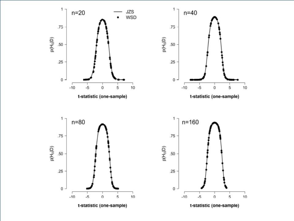
20. WSD t-test  The t-test can be implemented in WinBUGS.  We get close correspondence to Rouder et al.’s analytical t-test.  The WSD t-test can also be implemented for two-sample tests (in which the two groups can also have different variances).  Here we’ll focus on the problem that still plagues Dr. Smith…

21. Helping Dr. Smith (This Time for Real)  The Smith data (t = 0.79, p =.44)  This is a within-subject experiment, so we can subtract the recall scores (winter minus summer) and see whether the difference is zero or not.

22. NB: Rouder’s test also gives BF 01 = 6.08 Dr. Smith Data: Non-directional Test

23. Dr. Smith Data: SMM Directional Test This means that p(H 0 |D) is about 0.93 (in case H 0 and H 1 are equally likely a priori)

24. Dr. Smith Data: Directional Test Inconsistent with SMM’s prediction

25. Helping Dr. Smith (This Time for Real)  According to our t-test, the data are about 14 times more likely under the null hypothesis than under the SMM hypothesis.  This is generally considered strong evidence in favor of the null.  Note that we have quantified evidence in favor of the null, something that is impossible in p-value hypothesis testing.