1. DREAM PLAN IDEA IMPLEMENTATION 1

2. 2

3. 3 Introduction to Image Processing Dr. Kourosh Kiani Email: kkiani2004@yahoo.comkkiani2004@yahoo.com Email: Kourosh.kiani@aut.ac.irKourosh.kiani@aut.ac.ir Email: Kourosh.kiani@semnan.ac.irKourosh.kiani@semnan.ac.ir Web: www.kouroshkiani.comwww.kouroshkiani.com Present to: Amirkabir University of Technology (Tehran Polytechnic) & Semnan University

4. Lecture 05 4 Mask processing or Spatial filter

5.  Spatial Domain  Frequency Domain (i.e., uses Fourier Transform)

6.  Convert a given pixel value to a new pixel value based on some predefined function.

7.  Need to define: 1. Area shape and size 2. Operation output image

8. Area shape is typically defined using a rectangular mask. Area size is determined by mask size. e.g., 3x3 or 5x5 Mask size is an important parameter!

9.  Neighborhood operation work with values of the image pixels and corresponding values of a sub image.  The sub image is called:  Filter  Mask  Kernel  Template  Window  The values in a filter sub image are referred to as coefficients, rather than pixels.  Our focus will be on masks of odd sizes, e.g. 3x3, 5x5,…

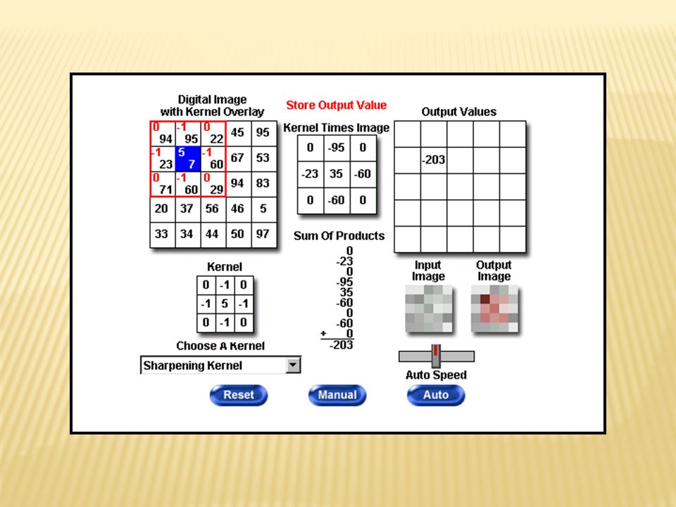
10.  Typically linear combinations of pixel values.  e.g., weight pixel values and add them together.  Different results can be obtained using different weights.  e.g., smoothing, sharpening, edge detection). mask

11. 0.5 00 0 000 mask 8 Modified image dataLocal image neighborhood 614 181 5310 1

13.  Correlation  Convolution

14.  A filtered image is generated as the center of the mask visits every pixel in the input image. g(i,j) h(i,j) f(i,j) filtered image n x n mask

15. 0 0 0 ……………………….0 Option 1: Zero padding Option 2: Wrap around Option 3: Reflection 0 0 0 1 2 3 4 5 0 0 0 4 10 16 22 22 1 2 3 * 3 4 5 1 2 3 4 5 1 2 3 4 5 19 10 16 22 23 5 3 2 1 1 2 3 4 5 5 4 3 2 7 10 16 22 27 5

18.  Commutative: A*B = B*A  Associative: (A*B)*C = A*(B*C)  Linear: A*(  B+  C)=  A*B+  A*B  Shift-Invariant A*B(x-x 0,y-y o )= (A*B) (x-x 0,y-y o )

19. 0 1 0 A(x)*  (x) = A(x) 0 0 0 0 1 0 0 0 0 A(x,y)*  (x,y) = A(x,y)

20.  Due to shift-invariance: A(x,y)*  (x-x 0,y-y 0 ) = A(x-x 0,y-y 0 ) 0 0 0 0 1 0 0 0 0 0 0 1  (x,y)  (x-1,y-1) 1 2 3 4 5 6 7 8 9 A * 0 0 0 0 0 1  (x-1,y-1) = 0 0 0 0 1 2 0 4 5 A(x-1,y-1) (Zero padding) 9 7 8 3 1 2 6 4 5 A(x-1,y-1) (Wrap around) =

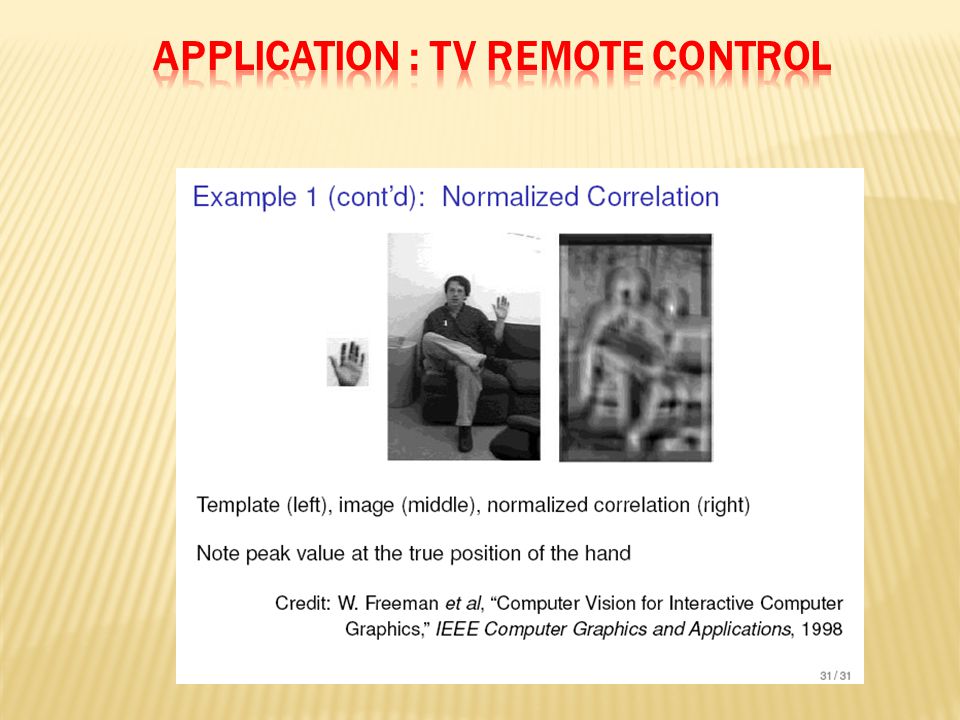
22.  Suppose x and y are two n-dimensional vectors:  The dot product of x with y is defined as:  Correlation generalizes the notion of dot product using vector notation: x y θ

23. cos(θ) measures the similarity between x and y Normalized correlation (i.e., divide by lengths)

24. Measure the similarity between images or parts of images. = mask

26. Traditional correlation cannot handle changes due to: size orientation shape (e.g., deformable objects). ?

27.  Same as correlation except that the mask is flipped, both horizontally and vertically. h * f = f * h Notation: 123 456 789 789 456 123 987 654 321 H V For symmetric masks (i.e., h(i,j)=h(-i,-j)), convolution is equivalent to correlation!

28. Correlation: Convolution:

30. A = [10 20 30;40 50 60;70 80 90] A = 10. 20. 30. 40. 50. 60. 70. 80. 90. H = [1 2 3;4 5 6;7 8 9] H = 1. 2. 3. 4. 5. 6. 7. 8. 9. Correlation result = (10 x 1) + (20 x 2) + (30 x 3) + (40 x 4) + (50 x 5) + (60 x 6) + (70 x 7) + (80 x 8) + (90 x 9) = 2850 Convolution and Correlation in Image Processing is quite similar except that the kernel are rotated 180 degree between these 2 operation. Convolution and Correlation in Image Processing

31. A = [10 20 30;40 50 60;70 80 90] A = 10. 20. 30. 40. 50. 60. 70. 80. 90. H = [1 2 3;4 5 6;7 8 9] H = 1. 2. 3. 4. 5. 6. 7. 8. 9. H180= 9 8 7 6 5 4 3 2 1 Convolution and Correlation in Image Processing Convolution result = (10 x 9) + (20 x 8) + (30 x 7) + (40 x 6) + (50 x 5) + (60 x 4) + (70 x 3) + (80 x 2) + (90 x 1) = 1650

32. In the real Image convolution and correlation, the kernel is sliding over every single pixel and performs above operation to form a new image Convolution and Correlation in Image Processing

39. A = [10 20 30;40 50 60;70 80 90] A = 10. 20. 30. 40. 50. 60. 70. 80. 90. H = [1 2 3;4 5 6;7 8 9] H = 1. 2. 3. 4. 5. 6. 7. 8. 9. corr_result = imfilter(A,H) corr_result = 1350. 1680. 1950. 2520. 2850. 3120. 3150. 3480. 3750. -->conv_result = imfilter(A,rot90(H,2)) conv_result = 750. 1020. 1350. 1380. 1650. 1980. 2550. 2820. 3150. Convolution and Correlation in Image Processing

40. Most of the time the choice of using the convolution and correlation is up to the preference of the users, and it is identical when the kernel is symmetrical. For example, a smoothing filter which is: Convolution and Correlation in Image Processing

41. 111 111 111 121 242 121 Standard average Weighted average

42. kk=imread(‘nice.jpg'); corr_result = imfilter(kk,H); imshow(corr_result)

43. Origin kk=imread(‘nice.jpg'); corr_result = imfilter(kk,H); imshow(corr_result) Blur

44. Origin kk=imread(‘nice.jpg'); corr_result = imfilter(kk,H); imshow(corr_result) Blur

45. Motion Blur Origin kk=imread(‘nice.jpg'); corr_result = imfilter(kk,H); imshow(corr_result) Motion blur is achieved by blurring in only 1 direction

46. Find Edges Origin kk=imread(‘nice.jpg'); corr_result = imfilter(kk,H); imshow(corr_result) A filter of 5x5 instead of 3x3 was chosen, because the result of a 3x3 filter is too dark on the current image. Note that the sum of all the elements is 0 now, which will result in a very dark image where only the edges it detected are colored.

47. Origin kk=imread(‘nice.jpg'); corr_result = imfilter(kk,H); imshow(corr_result) Sharpen

48. kk=imread(‘nice.jpg'); corr_result = imfilter(kk,H); imshow(corr_result) Extra Edge Here's a filter that shows the edges excessively Origin

49. kk=imread(‘nice.jpg'); corr_result = imfilter(kk,H); imshow(corr_result) Origin Emboss An emboss filter gives a 3D shadow effect to the image, the result is very useful for a bumpmap of the image

50. 30 10 20 10 25 250 20 25 30 10, 10, 20, 20, 25, 25, 30, 30, 250 min max  Min filter:  Max filter Min & Max Filters

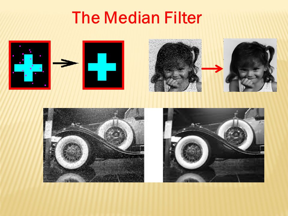
51. 30 10 20 10 25 250 20 25 30 10, 10, 20, 20, 25, 25, 30, 30, 250 median The Median Filter

53. Noisy image 3x3 average 5x5 average 7x7 average median

54.  Filtering is often used to remove noise from images  Sometimes a median filter works better than an averaging filter Original Image With Noise Image After Averaging Filter Image After Median Filter

55. Original Gaussian noise salt & pepper

56. Median filter 3x3 window Gaussian blur std=1.5 Salt & Pepper Noise:

57. Median filter 5x5 window Gaussian blur std=1.5 Gaussian Noise:

58. Noise from Glass effectRemove noise by median filter

59.  Separable Filter

60.  Convolution with self is another Gaussian Special case: convolving two times with Gaussian kernel of width is equivalent to convolving once with kernel of width * =

61. Separable kernel: a 2D Gaussian can be expressed as the product of two 1D Gaussians.

62.  2D Gaussian convolution can be implemented more efficiently using 1D convolutions:

63. row get a new image I r Convolve each column of I r with g

64. 2D convolution (center location only) The filter factors into a product of 1D filters: Perform convolution along rows: Followed by convolution along the remaining column: * * = = O(n 2 ) O(2n)=O(n)

65.  Complexity of non-separable filter: N 2  Complexity of separable filter: 2N

66.  Depends on the application.  Usually by sampling certain functions and their derivatives. Gaussian 1 st derivative of Gaussian 2 nd derivative of Gaussian Good for image smoothing Good for image sharpening

67.  Sum of weights affects overall intensity of output image.  Positive weights one  Normalize them such that they sum to one.  Both positive and negative weights zero  Should sum to zero (but not always) 1/91/16

68. Idea: replace each pixel by the average of its neighbors. Useful for reducing noise and unimportant details. The size of the mask controls the amount of smoothing.

69.  Trade-off: noise vs blurring and loss of detail. 3x35x57x7 15x1525x25 original

70.  Idea: replace each pixel by a weighted average of its neighbors  Mask weights are computed by sampling a Gaussian function Note: weight values decrease with distance from mask center!

71.  The Gaussian kernel is separable and symmetric.  To construct the kernel we must sample and quantize! (basically, we “image” the function)  The kernel below is an example where sigma = 1. 14741 41628164 72849287 41628164 14741

72. mask size depends on σ : σ determines the degree of smoothing! σ=3

73. = 30 pixels= 1 pixel = 5 pixels = 10 pixels

74. Averaging Gaussian

75.  Idea: compute intensity differences in local image regions.  Useful for emphasizing transitions in intensity (e.g., in edge detection). 1 st derivative of Gaussian

77. Zooming as a Convolution Application Example 1 3 2 4 5 6 Zero interlace 1 0 3 0 2 0 0 0 0 4 0 5 0 6 0 0 0 0 Convolve 1 1 1 The value of a pixel in the enlarged image is the average of the value of around pixels. The difference between insert 0 and original value of pixels is “smoothed” by convolution Original Image (1+0+3+0+0+0+4+0+5) ÷(1+1+1+1+1+1+1+1+1) = 13/9

78. Zooming as a Convolution Application Example

80. Questions? Discussion? Suggestions ?

81. 81