1. Keynesian Model of the trade balance TB & income Y. Key assumption: P fixed =>. Mundell-Fleming model Key additional assumption: international capital flows KA respond to interest rates i. LECTURE 2: The Mundell-Fleming Model with a Fixed Exchange Rate Questions: Effect of fiscal expansion or other . Effect of monetary expansion  /.

2. ALTERNATE APPROACHES TO DETERMINATION OF EXTERNAL BALANCE  Elasticities Approach to the Trade Balance  Keynesian Approach to the Trade Balance  Mundell-Fleming Model of the Balance of Payments  Monetary Approach to the Balance of Payments  NonTraded Goods or Dependent-Economy Model of the Trade Balance  Intertemporal Approach to the Current Account

3. KEYNESIAN MODEL OF THE TRADE BALANCE Import demand is a function of the exchange rate & income. The same for exports: => TB = X(E, Y*) – IM(E, Y), where IM is here defined to be import spending expressed in domestic terms.. If the domestic country is small, Y* is exogenous; drop it for simplicity. Rewrite TB =. and we assume the Marshall-Lerner condition holds:. Notationally, we embody all E effects (whether via exports or imports) in ;

4. STYLIZED J-CURVES With instantaneous pass-through to import prices With delayed pass-through to import prices

5. Empirical estimates of sensitivity of exports and imports to E & Y For empirical purposes, we estimate by OLS regression – with allowance for lags, giving J-curve; – controlling for income Y & Y* as well as E, – shown in logs, giving parameters as: price elasticities & income elasticities. Illustration: Marquez (2002) finds for most Asian countries: – Marshall-Lerner condition holds, after a couple of years, and – income elasticities are in the 1.0-2.0 range. log X

6. Estimated price elasticities (LR) satisfy the Marshall-Lerner Condition. Estimated income elasticities are mostly between 1.0 - 2.0.

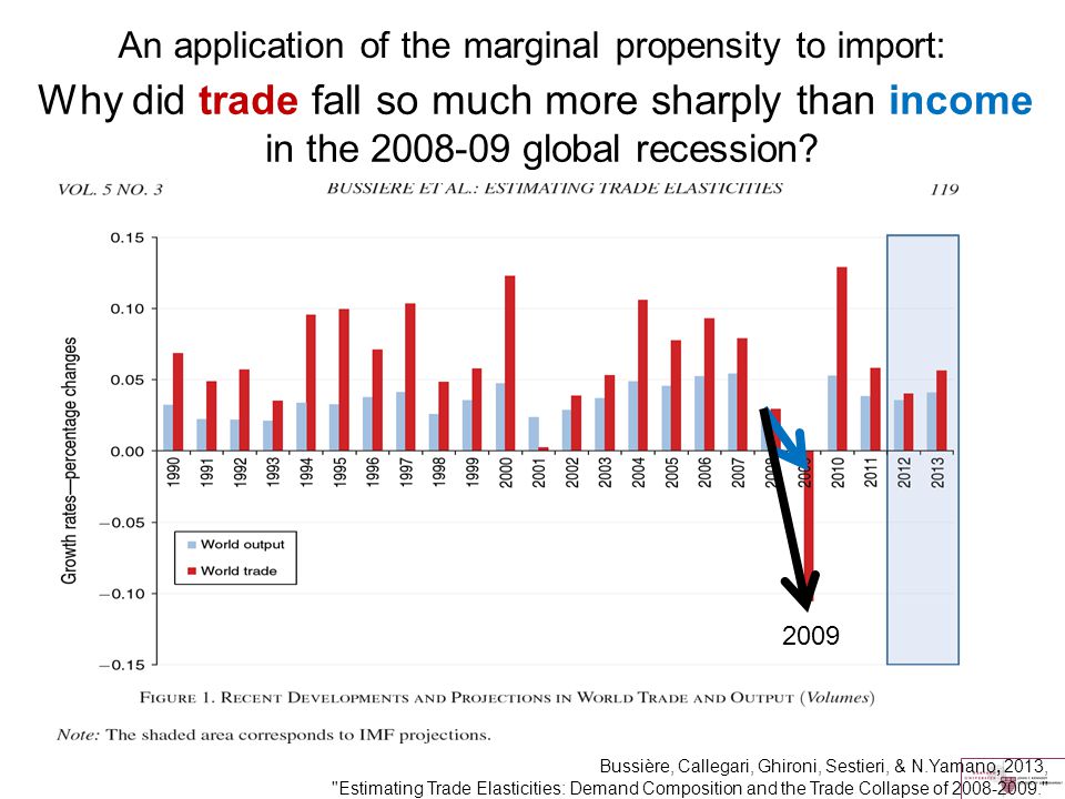
7. An application of the marginal propensity to import: Bussière, Callegari, Ghironi, Sestieri, & N.Yamano, 2013, "Estimating Trade Elasticities: Demand Composition and the Trade Collapse of 2008-2009." Why did trade fall so much more sharply than income in the 2008-09 global recession? 2009

8. Bussière, Callegari, Ghironi, Sestieri, & Yamano, 2013, "Estimating Trade Elasticities: Demand Composition and the Trade Collapse of 2008-09." Why did trade fall so sharply in the 2008-09 global recession? The usual explanations involve trade credit, inventories, and trade in intermediate inputs.

9. Behavior of real components of GDP in the 2008-09 recession Demand, adjusted for import-intensity GDP Investment Imports & Exports Bussière, Callegari, Ghironi, Sestieri, & N.Yamano, "Estimating Trade Elasticities: Demand Composition and the Trade Collapse of 2008-2009.“ Bussière et al (2013) argue that Investment, which declined much more in 2009 than the other components of GDP, has a higher marginal propensity to import than the other components.

10. Trade Balance = TB = (E) – mY. Aggregate output = domestic Aggregate Demand + net foreign demand: Y = A(i, Y) + TB(E, Y), More specifically, let A(i, Y) = Ā - b(i) + cY, where the function -b( ) captures the negative effect of the interest rate i on investment spending, consumer durables, etc. Solve to get the IS curve: where s  1 – c is the marginal propensity to save. where and. Combining equations, Y =

11. IS curve: An inverse relationship between i and Y consistent with the equilibrium that supply = demand in the goods market. An increase in spending, Ā, e.g., a fiscal expansion, shifts IS to the right by the multiplier 1/(s+m).

12. The overall balance of payments is given by BP = TB + KA, where  , the degree of capital mobility > 0. We want to graph BP = 0. Solve for the interest rate: The Mundell-Fleming model introduces capital flows: slope = m/

13. A monetary expansion shifts the LM curve to the right. LM´ Do central banks actually set M? Supposedly they set M1, in the 1980s heyday of monetarism. Also the monetary base made a comeback after 2008: Quantitative Easing. Normally they think in terms of setting i. Still, the role of the LM equation can be taken by a Taylor Rule, which describes central banks as setting i in response to Y & inflation. →

14. Appendix: Causes of Developing Country BoP Surpluses 2003-08 & 2010-13 Strong economic performance (especially China & India) -- IS shifts right. Easy monetary policy in US and other major industrialized countries (low i*) -- BP shifts down. Big boom in mineral & agricultural commodities (esp. Africa & Latin America) -- BP shifts right.

15. Causes of BoP Surpluses in Developing Countries 1990-1997, 2003-08 & 2010-13 I.“Pull” Factors (internal causes) 1. Monetary stabilization => LM shifts up 2. Removal of capital controls => κ rises 3. Spending boom => IS shifts out/up II. “Push” Factors (external causes) 1.Low interest rates in rich countries => i* down => 2.Boom in export markets => BP shifts down out }