1. Search Search plays a key role in many parts of AI. These algorithms provide the conceptual backbone of almost every approach to the systematic exploration of alternatives. There are four classes of search algorithms, which differ along two dimensions: –First, is the difference between uninformed (also known as blind) search and then informed (also known as heuristic) searches. Informed searches have access to task-specific information that can be used to make the search process more efficient. –The other difference is between any solution searches and optimal searches. Optimal searches are looking for the best possible solution while any- path searches will just settle for finding some solution.

2. Graphs Graphs are everywhere; E.g., think about road networks or airline routes or computer networks. In all of these cases we might be interested in finding a path through the graph that satisfies some property. It may be that any path will do or we may be interested in a path having the fewest "hops" or a least cost path assuming the hops are not all equivalent.

3. Romania graph

4. Formulating the problem On holiday in Romania; currently in Arad. Flight leaves tomorrow from Bucharest. Formulate goal: –be in Bucharest Formulate problem: –states: various cities –actions: drive between cities Find solution: –sequence of cities, e.g., Arad, Sibiu, Fagaras, Bucharest

5. Another graph example However, graphs can also be much more abstract. A path through such a graph (from a start node to a goal node) is a "plan of action" to achieve some desired goal state from some known starting state. It is this type of graph that is of more general interest in AI.

6. Problem solving One general approach to problem solving in AI is to reduce the problem to be solved to one of searching a graph. To use this approach, we must specify what are the states, the actions and the goal test. A state is supposed to be complete, that is, to represent all the relevant aspects of the problem to be solved. We are assuming that the actions are deterministic, that is, we know exactly the state after the action is performed.

7. Goal test In general, we need a test for the goal, not just one specific goal state. –So, for example, we might be interested in any city in Germany rather than specifically Frankfurt. Or, when proving a theorem, all we care is about knowing one fact in our current data base of facts. –Any final set of facts that contains the desired fact is a proof.

8. Vacuum cleaner?

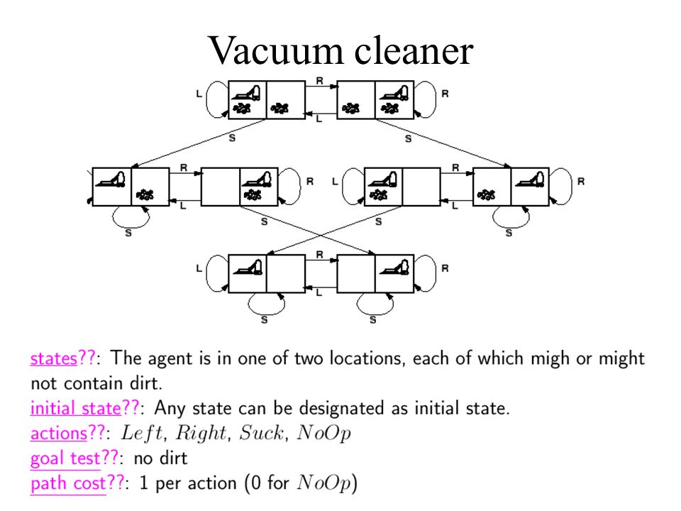
9. Vacuum cleaner

11. Formally… A problem is defined by four items: 1.initial state e.g., "at Arad" 2.actions and successor function S: = set of action-state tuples –e.g., S(Arad) = {(goZerind, Zerind), (goTimisoara, Timisoara), (goSilbiu, Silbiu)} 3.goal test, can be –explicit, e.g., x = "at Bucharest" –implicit, e.g., Checkmate(x) 4.path cost (additive) –e.g., sum of distances, or number of actions executed, etc. –c(x,a,y) is the step cost, assumed to be 0 A solution is a sequence of actions leading from the initial state to a goal state

12. Example: The 8-puzzle states? actions? goal test? path cost?

13. Example: The 8-puzzle states? locations of tiles actions? move blank left, right, up, down goal test? = goal state (given) path cost? 1 per move

14. Romania graph

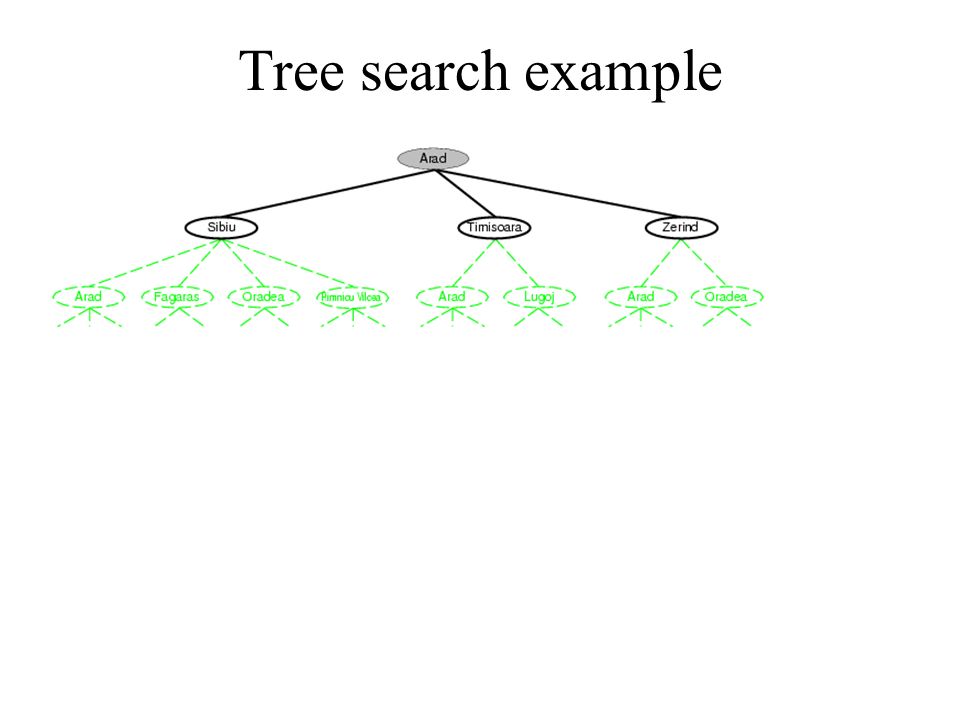
15. Tree search example

18. Tree search algorithms Basic idea: –Exploration of state space by generating successors of already-explored states (i.e. expanding states)

19. (

20. Data type node: components : STATE, PARENT_NODE, OPERATOR, DEPTH, PATH_COST components : STATE, PARENT_NODE, OPERATOR, DEPTH, PATH_COST

21. Function GENERAL-SEARCH ( problem,QUEUING_FN ) returns a solution or failure nodes MAKE_QUEUE (MAKE_NODE (INITIAL_STATE [problem ] )) nodes MAKE_QUEUE (MAKE_NODE (INITIAL_STATE [problem ] )) Loop do if nodes is empty then return failure if nodes is empty then return failure node REMOVE_FRONT (nodes ) node REMOVE_FRONT (nodes ) if GOAL_TEST [problem ] applied to STATE ( node ) succeeds then return node if GOAL_TEST [problem ] applied to STATE ( node ) succeeds then return node nodes QUEUING_FN (nodes, EXPAND (node,OPERATORS [problem ] )) nodes QUEUING_FN (nodes, EXPAND (node,OPERATORS [problem ] ))End

22. Function SIMPLE-PROBLEM-SOLVING-AGENT (percept) returns an action Inputs: percept, a percept Static: seq, an action sequence, initially empty state, some description of the current world state goal, a goal, initially null problem, a problem formulation State UPDATE-STATE(state,percept) If seq is empty then do goal FORMULATE-GOAL(state) problem FORMULATE-PROBLEM(state,goal) seq SEARCH(problem) action FIRST(seq) seq REST(seq) Return action

23. Function Tree-Search(problem,fringe) returns a solution, or failure fringeInsert(MAKE-NODE(INITIAL-STATE[problem]),fringe) loop do if Empty?(fringe) then return failure node REMOVE-FIRST(fringe) if GOAL-TEST[problem] applied to STATE[node] succeeds then return SOLUTION(node) fringe INSERT-ALL(EXPAND(node,problem),fringe) Function EXPAND(node,problem) returns a set of nodes successors the empty set For each(action,result)in SUCCESSOR-FN[problem](STATE[node]) do s a new node STATE[s] result PARENT-NODE[s] node ACTION[s] action PATH-COST[s] PATH-COST[node]+STEP-COST(node,action,s) DEPTH[s] DEPTH[node]+1 add s to successors return successors

24. Search strategies A search strategy is defined by picking the order of node expansion Strategies are evaluated along the following dimensions: –completeness: does it always find a solution if one exists? –time complexity: number of nodes generated –space complexity: maximum number of nodes in memory –optimality: does it always find a least-cost solution? Time and space complexity are measured in terms of –b: maximum branching factor of the search tree –d: depth of the least-cost solution –m: maximum depth of the state space

25. Uninformed search strategies Uninformed do not use information relevant to the specific problem. Breadth-first search Uniform-cost search Depth-first search Depth-limited search Iterative deepening search Bidirectional search

26. Function BREADTH_FIRST_SEARCH ( problem ) return a solution or failure return GENERAL_SEARCH (problem,ENQUEUE_AT_END

27. Breadth-first search TreeSearch(problem, FIFO-QUEUE()) results in a breadth-first search. The FIFO queue puts all newly generated successors at the end of the queue, which means that shallow nodes are expanded before deeper nodes. –I.e. Pick from the fringe to expand the shallowest unexpanded node

28. Breadth-first search Expand shallowest unexpanded node Implementation: –fringe is a FIFO queue, i.e., new successors go at end

29. Breadth-first search Expand shallowest unexpanded node Implementation: –fringe is a FIFO queue, i.e., new successors go at end

30. Breadth-first search Expand shallowest unexpanded node Implementation: –fringe is a FIFO queue, i.e., new successors go at end

31. Properties of breadth-first search Complete? –Yes (if b is finite) Time? –1+b+b 2 +b 3 +… +b d + b(b d -1) = O(b d+1 ) Space? –O(b d+1 ) (keeps every node in memory) Optimal? –Yes (if cost is a non-decreasing function of depth, e.g. when we have 1 cost per step)

32. DepthNodesTimeMemory 011 millisecodns100 bytes 2111.1 sec11 kilobytes 411,11111 sec1 Megabyte 610 6 18 min111 Megabyte 810 8 31 hours11Gigabyte 1010 128 days1 Terabyte 1210 12 35 years111 Terabyte 1410 14 3500 years11111 Terabyte Suppose b=10, 1000 nodes/sec, 100 bytes/node

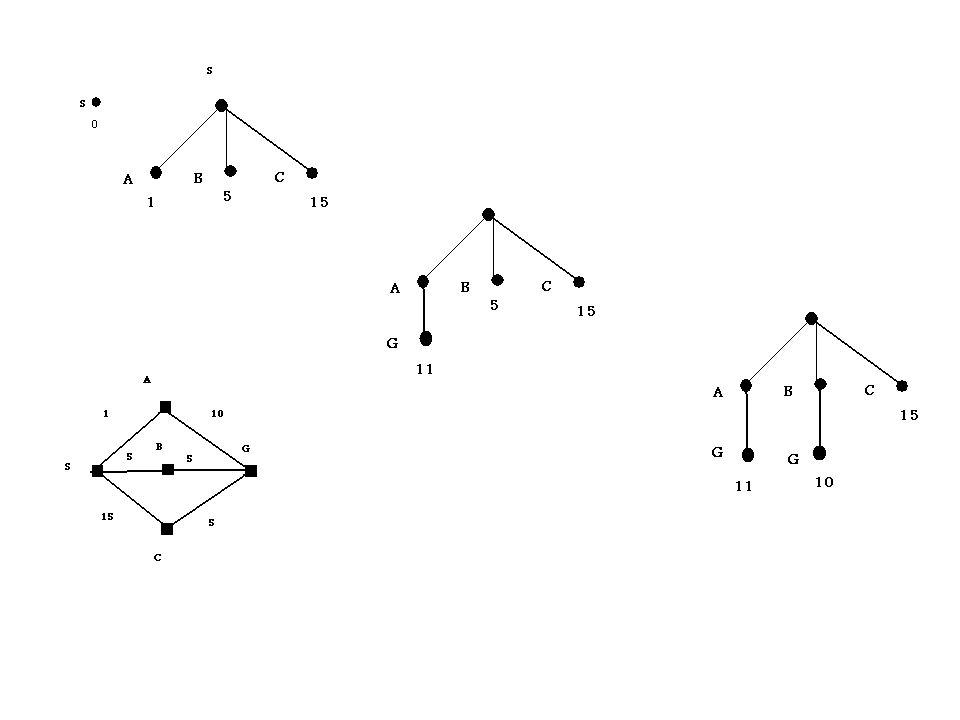
33. Uniform-cost search Expand least-cost unexpanded node. The algorithm expands nodes in order of increasing path cost. Therefore, the first goal node selected for expansion is the optimal solution. Implementation: –fringe = queue ordered by path cost (priority queue) Equivalent to breadth-first if step costs all equal Complete? Yes, if step cost ε (I.e. not zero) Time? number of nodes with g cost of optimal solution, O(b C*/ ε ) where C * is the cost of the optimal solution Space? Number of nodes with g cost of optimal solution, O(b C*/ ε ) Optimal? Yes – nodes expanded in increasing order of g(n)

35. Depth-first search Expand deepest unexpanded node Implementation: –fringe = LIFO queue, i.e., put successors at front

36. Depth-first search Expand deepest unexpanded node Implementation: –fringe = LIFO queue, i.e., put successors at front

37. Depth-first search Expand deepest unexpanded node Implementation: –fringe = LIFO queue, i.e., put successors at front

38. Depth-first search Expand deepest unexpanded node Implementation: –fringe = LIFO queue, i.e., put successors at front

39. Depth-first search Expand deepest unexpanded node Implementation: –fringe = LIFO queue, i.e., put successors at front

40. Depth-first search Expand deepest unexpanded node Implementation: –fringe = LIFO queue, i.e., put successors at front

41. Depth-first search Expand deepest unexpanded node Implementation: –fringe = LIFO queue, i.e., put successors at front

42. Depth-first search Expand deepest unexpanded node Implementation: –fringe = LIFO queue, i.e., put successors at front

43. Depth-first search Expand deepest unexpanded node Implementation: –fringe = LIFO queue, i.e., put successors at front

44. Depth-first search Expand deepest unexpanded node Implementation: –fringe = LIFO queue, i.e., put successors at front

45. Depth-first search Expand deepest unexpanded node Implementation: –fringe = LIFO queue, i.e., put successors at front

46. Depth-first search Expand deepest unexpanded node Implementation: –fringe = LIFO queue, i.e., put successors at front

47. Properties of depth-first search Complete? No: fails in infinite-depth spaces, spaces with loops –Modify to avoid repeated states along path complete in finite spaces Time? O(b m ): terrible if m is much larger than d – but if solutions are dense, may be much faster than breadth-first Space? O(bm), i.e., linear space! Optimal? No

48. Function DEPTH_FIRST_SEARCH ( problem ) return a solution or failure return GENERAL_SEARCH (problem,ENQUEUE_AT_FRONT ) DEPTH_FIRST_SEARCH 1.List s 2.if List = null then fail, stop 3.n First (List) 4.if n = GOAL then success, stop 5. List Tail ( List ) 6. Clist Expand( n ) 7. List Append (Clist, List ) 8. Goto 2 Nilsson Algorithm

49. DepthLimitedSearch (int limit) { stackADT fringe; insert root into the fringe do { if (Empty(fringe)) return NULL; /* Failure */ nodePT = Pop(fringe); if (GoalTest(nodePT->state)) return nodePT; /* Expand node and insert all the successors */ if (nodePT->depth < limit) insert into the fringe Expand(nodePT) } while (1); } Depth-limited search

50. Iterative deepening Search Function ITERATIVE_DEEPING_SEARCH( problem ) returns a solution sequence or failure inputs: problem, a problem for depth 0 to do if DEPTH_LIMITED_SEARCH ( problem, depth ) succeeds then return its result end return failure

51. Iterative deepening search l =0

52. Iterative deepening search l =1

53. Iterative deepening search l =2

54. Iterative deepening search l =3

55. Iterative deepening search Number of nodes generated in a breadth-first search to depth d with branching factor b: N BFS = b 0 + b 1 + b 2 + … + b d-2 + b d-1 + b d Number of nodes generated in an iterative deepening search to depth d with branching factor b: N IDS = (d+1)b 0 + d b 1 + (d-1)b 2 + … + 3b d-2 +2b d-1 + 1b d For b = 10, d = 5, –N BFS = 1 + 10 + 100 + 1,000 + 10,000 + 100,000 = 111,111 –N IDS = 6 + 50 + 400 + 3,000 + 20,000 + 100,000 = 123,456 Overhead = (123,456 - 111,111)/111,111 = 11%

56. Properties of iterative deepening search Complete? Yes Time? (d+1)b 0 + d b 1 + (d-1)b 2 + … + b d = O(b d ) Space? O(bd) Optimal? Yes, if step cost = 1

57. Which Direction Should We Search? Our choices: Forward, backwards, or bidirectional The issues: How many start and goal states are there? Branching factors in each direction How much work is it to compare states?

58. Summary of algorithms Criterion Breadth- First Uniform- Cost Depth- First Depth- Limited Iterative Deepening Bidirectional (if applicable) Complete? Yes No Yes, If l d Yes Time b d b m b l b d b d/2 Space b d bm bl bd b d/2 Optimal? Yes No Yes

59. Repeated states Failure to detect repeated states can turn a linear problem into an exponential one!

60. Graph search