Download presentation
Presentation is loading. Please wait.

1
Markets in Uncertainty: Risk, Gambling, and Information Aggregation
a tutorial by David M. Pennock Michael P. Wellman dpennock.com ai.eecs.umich.edu/people/wellman presented at the 19th National Conference on Artificial Intelligence, July 2004, San Jose, CA, USA MP1-1

2
Outline Overview tour 15 min What is a “market in uncertainty”?
Background min Single agent perspective Subjective probability Utility, risk, and risk aversion Decision making under uncertainty Multiagent perspective Trading/allocating risk Pareto optimality Securities: Markets in uncertainty AAAI’04 July 2004 MP1-2

3
Outline Mechanisms, examples and empirical studies 45 min
What & how: Instruments & mechanisms Real-money markets: Examples & evaluations Iowa Electronic Market Options TradeSports: Effects of war Horse racing, sports betting Play-money markets AAAI’04 July 2004 MP1-3

4
Outline Lab experiments and theory 20 min
Laboratory experiments, field tests Theoretical underpinnings Rational expectations Efficient markets hypothesis No-Trade Theorems Information aggregation AAAI’04 July 2004 MP1-4

5
Outline Characterizing information 20 min aggregation
Market as an opinion pool Market as a “composite agent” Market belief, utility Market Bayesian updates Market adaptation, dynamics Paradoxes, impossibilities Opinion pool impossibilities Composite agent non-existence AAAI’04 July 2004 MP1-5

6
Outline Computational aspects 60 min Legal issues; miscellaneous 5 min
Combinatorics Compact securities markets Combinatorial securities markets Compound securities markets Market scoring rules Dynamic pari-mutuel market Policy Analysis Market Distributed market computation Legal issues; miscellaneous 5 min Discussion, Q&A min AAAI’04 July 2004 MP1-6

7
What is a “market in uncertainty” ?
1. Overview tour What is a “market in uncertainty” ?

8
A market in uncertainty
Take a random variable, e.g. Turn it into a financial instrument payoff = realized value of variable 2004 CA Earthquake? US’04Pres = Bush? = 6 ? = 6 $1 if 6 $0 if I am entitled to: AAAI’04 July 2004 MP1-8

9
Aside: Terminology Key aspect: payout is uncertain
Called variously: asset, security, contingent claim, derivative (future, option), stock, prediction market, information market, gamble, bet, wager, lottery Historically mixed reputation Esp. gambling aspect A time when options were frowned upon But when regulated serve important social roles... AAAI’04 July 2004 MP1-9
, stock, prediction market, information market, gamble, bet, wager, lottery. Historically mixed reputation. Esp. gambling aspect. A time when options were frowned upon. But when regulated serve important social roles... AAAI’04 July MP1-9.")
10
Why? Reason 1 Get information
price expectation of random variable (in theory, lab experiments, empirical studies, ...more later) Do you have a random variable whose expectation you’d like to know? A market in uncertainty can probably help AAAI’04 July 2004 MP1-10
 Do you have a random variable whose expectation you’d like to know A market in uncertainty can probably help. AAAI’04 July MP1-10.")
11
Why? Reason 1: Information
“Information market”: financial mechanism designed to obtain estimates of expectations of random variables Easy as 1, 2, 3: Take a random variable whose expectation you’d like to know Turn it into a financial instrument (payoff= realized value of variable) Open a market in the financial instrument price(t) Et[X] (in many cases, ... more later) AAAI’04 July 2004 MP1-11
 Open a market in the financial instrument. price(t) Et[X] (in many cases, ... more later) AAAI’04 July MP1-11.")
12
Getting information = 6 $1 if 6 $0 if
Non-market approach: ask an expert How much would you pay for this? A: $5/36 $0.1389 caveat: expert is knowledgeable caveat: expert is truthful caveat: expert is risk neutral, or ~ RN for $1 caveat: expert has no significant outside stakes = 6 $1 if 6 $0 if I am entitled to: AAAI’04 July 2004 MP1-12

13
Getting information Non-market approach: pay an expert
Ask the expert for his report r of the probability P( ) Offer to pay the expert $100 + log r if $100 + log (1-r) if It so happens that the expert maximizes expected profit by reporting r truthfully caveat: expert is knowledgeable caveat: expert is truthful caveat: expert is risk neutral, or ~ RN caveat: expert has no significant outside stakes = 6 = 6 “logarithmic scoring rule”, a “proper” scoring rule 6 AAAI’04 July 2004 MP1-13
 Offer to pay the expert. $100 + log r if. $100 + log (1-r) if. It so happens that the expert maximizes expected profit by reporting r truthfully. caveat: expert is knowledgeable. caveat: expert is truthful. caveat: expert is risk neutral, or ~ RN. caveat: expert has no significant outside stakes. = 6. = 6. logarithmic scoring rule , a proper scoring rule. 6. AAAI’04 July MP1-13.")
14
Getting information = 6 $1 if 6 $0 if = 6
Market approach: “ask” the public—experts & non-experts alike—by opening a market: Let any person i submit a bid order: an offer to buy qi units at price pi Let any person j submit an ask order: an offer to sell qj units at price pj (if you sell 1 unit, you agree to pay $1 if ) Match up agreeable trades (many poss. mechs...) = 6 $1 if 6 $0 if I am entitled to: = 6 AAAI’04 July 2004 MP1-14
 Match up agreeable trades (many poss. mechs...) = 6. $1 if. 6. $0 if. I am entitled to: = 6. AAAI’04 July MP1-14.")
15
Getting information = 6 $1 if 6 $0 if
Market approach: “ask” the public—experts & non-experts alike—by opening a market: If, at any time, for any bidder i and ask-er j, pi > pj, then i&j trade min(qi,qj) units at price {pj,pi} In equilibrium (no trades) max bid pi < min ask pj = “bid-ask spread” bounds aggregate public opinion of expectation = 6 $1 if 6 $0 if I am entitled to: AAAI’04 July 2004 MP1-15
 units at price {pj,pi} In equilibrium (no trades) max bid pi < min ask pj = bid-ask spread bounds aggregate public opinion of expectation. = 6. $1 if. 6. $0 if. I am entitled to: AAAI’04 July MP1-15.")
16
Aside: Mechanism alternatives
This is the continuous double auction (CDA) Many other market & auction mechanisms work: call market pari-mutuel market market scoring rules CDA w/ market maker Vegas bookmaker, others Key: Market price = aggregate estimate of expected value [Hanson 2002] AAAI’04 July 2004 MP1-16
 Many other market & auction mechanisms work: call market. pari-mutuel market. market scoring rules. CDA w/ market maker. Vegas bookmaker, others. Key: Market price = aggregate estimate of expected value. [Hanson 2002] AAAI’04 July MP1-16.")
17
(Real) Great expectations
For dice example, no need for market: E[x] is known; no one should disagree Real power comes for non-obvious expectations of random variables, e.g. I am entitled to: $1 if ; $0 otherwise I am entitled to: $x if interest rate = x on Jan 1, 2004 AAAI’04 July 2004 MP1-17

18
$max(0,x-k) if MSFT = x on Jan 1, 2004
I am entitled to: $max(0,x-k) if MSFT = x on Jan 1, 2004 call option I am entitled to: $f(future weather) weather derivative I am entitled to: Bin Laden captured $1 if ; $0 otherwise I am entitled to: $1 if Kansas beats Marq. by > 4.5 points; $0 otherw. AAAI’04 July 2004 MP1-18
 if MSFT = x on Jan 1, call option. I am entitled to: $f(future weather) weather derivative. I am entitled to: Bin Laden captured. $1 if ; $0 otherwise. I am entitled to: $1 if Kansas beats Marq. by > 4.5 points; $0 otherw. AAAI’04 July MP1-18.")
20
IPO http://www.biz.uiowa.edu/iem http://www.wsex.com/
AAAI’04 July 2004 MP1-20

21
Play money; Real expectations
AAAI’04 July 2004 MP1-21

22
Cancer cured by 2010 Machine Go champion by 2020
Cancer cured by 2010 Machine Go champion by 2020

23
Does it work? Yes... Evidence from real markets, laboratory experiments, and theory indicate that markets are good at gathering information from many sources and combining it appropriately; e.g.: Markets like the Iowa Electronic Market predict election outcomes better than polls [Forsythe 1992, 1999][Oliven 1995][Rietz 1998][Berg 2001][Pennock 2002] Futures and options markets rapidly incorporate information, providing accurate forecasts of their underlying commodities/securities [Sherrick 1996][Jackwerth 1996][Figlewski 1979][Roll 1984][Hayek 1945] Sports betting markets provide accurate forecasts of game outcomes [Gandar 1998][Thaler 1988][Debnath EC’03][Schmidt 2002] AAAI’04 July 2004 MP1-23

24
Does it work? Yes... E.g. (cont’d):
Laboratory experiments confirm information aggregation [Plott 1982;1988;1997][Forsythe 1990][Chen, EC-2001] And field tests [Plott 2002] Theoretical underpinnings: “rational expectations” [Grossman 1981][Lucas 1972] Procedural explanation: agents learn from prices [Hanson 1998][Mckelvey 1986][Mckelvey 1990][Nielsen 1990] Proposals to use information markets to help science [Hanson 1995], policymakers, decision makers [Hanson 1999], government [Hanson 2002], military [DARPA FutureMAP, PAM] Even market games work! [Servan-Schreiber 2004][Pennock 2001] AAAI’04 July 2004 MP1-24

25
Why? Reason 2 Manage risk If is horribly terrible for you Buy a bunch of and if happens, you are compensated = 6 = 6 $1 if 6 $0 if I am entitled to: = 6 AAAI’04 July 2004 MP1-25

26
Why? Reason 2 Manage risk If is horribly terrible for you Buy a bunch of and if happens, you are compensated I am entitled to: $1 if $0 if AAAI’04 July 2004 MP1-26

27
The flip-side of prediction: Hedging (Reason 2)
Allocate risk (“hedge”) insured transfers risk to insurer, for $$ farmer transfers risk to futures speculators put option buyer hedges against stock drop; seller assumes risk Aggregate information price of insurance prob of catastrophe OJ futures prices yield weather forecasts prices of options encode prob dists over stock movements market-driven lines are unbiased estimates of outcomes IEM political forecasts AAAI’04 July 2004 MP1-27
 insured transfers risk to insurer, for $$ farmer transfers risk to futures speculators. put option buyer hedges against stock drop; seller assumes risk. Aggregate information. price of insurance prob of catastrophe. OJ futures prices yield weather forecasts. prices of options encode prob dists over stock movements. market-driven lines are unbiased estimates of outcomes. IEM political forecasts. AAAI’04 July MP1-27.")
28
Reason 2: Manage risk What is insurance?
A bet that something bad will happen! E.g., I’m betting my insurance co. that my house will burn down; they’re betting it won’t. Note we might agree on P(burn)! Why? Because I’ll be compensated if the bad thing does happen A risk-averse agent will seek to hedge (insure) against undesirable outcomes AAAI’04 July 2004 MP1-28
! Why Because I’ll be compensated if the bad thing does happen. A risk-averse agent will seek to hedge (insure) against undesirable outcomes. AAAI’04 July MP1-28.")
29
E.g. stocks, options, futures, insurance, ..., sports bets, ...
Allocate risk (“hedge”) insured transfers risk to insurer, for $$ farmer transfers risk to futures speculators put option buyer hedges against stock drop; seller assumes risk sports bet may hedge against other stakes in outcome Aggregate information price of insurance prob of catastrophe OJ futures prices yield weather forecasts prices of options encode prob dists over stock movements market-driven lines are unbiased estimates of outcomes IEM political forecasts AAAI’04 July 2004 MP1-29
 insured transfers risk to insurer, for $$ farmer transfers risk to futures speculators. put option buyer hedges against stock drop; seller assumes risk. sports bet may hedge against other stakes in outcome. Aggregate information. price of insurance prob of catastrophe. OJ futures prices yield weather forecasts. prices of options encode prob dists over stock movements. market-driven lines are unbiased estimates of outcomes. IEM political forecasts. AAAI’04 July MP1-29.")
30
Examples I buy MSFT stock at s. I’m afraid it will go down. I buy a put option that pays Max[0,k-s] – k is “strike” price. If s goes down below k, my stock investment goes down, but my option investment goes up to compensate I’m a farmer. I’m afraid corn prices will go too low. I buy corn futures to lock in a price today. AAAI’04 July 2004 MP1-30

31
Examples I own a house in CA. I’m afraid of earthquakes. I pay an insurance premium so that, if an earthquake happens, I am compensated. I am an Oscar-nominated actor. I’m afraid I’m going to lose. I bet against myself on an offshore gambling site. If I do lose, I am compensated. (Except that the offshore site disappears and refuses to pay…) AAAI’04 July 2004 MP1-31
 AAAI’04 July MP1-31.")
32
What am I buying? When you hedge/insure, you pay to reduce the unpredictability of future wealth Risk-aversion: All else being equal, prefer certainty to uncertainty in future wealth Typically, a less risk-averse party (e.g., huge insurance co, futures speculator) assumes the uncertainty (risk) in return for an expected profit AAAI’04 July 2004 MP1-32
 assumes the uncertainty (risk) in return for an expected profit. AAAI’04 July MP1-32.")
33
On hedging and speculating
Hedging is an act to reduce uncertainty Speculating is an act to increase expected future wealth A given agent engages in a (largely inseparable) mixture of the two Both can be encoded together as a maximization of expected utility, where utility is a function of wealth, ... more later AAAI’04 July 2004 MP1-33
 mixture of the two. Both can be encoded together as a maximization of expected utility, where utility is a function of wealth, ... more later. AAAI’04 July MP1-33.")
34
On trading Why would two parties agree to trade in a “market in uncertainty”? They disagree on expected values (prob’s) They differ in their risk attitude or exposure – they trade to reallocate risk Both (most likely) Aside: legality is murky, though generally (2) is legal in the US while (1) often is not. In reality, it is nearly impossible to differentiate. AAAI’04 July 2004 MP1-34
 Aside: legality is murky, though generally (2) is legal in the US while (1) often is not. In reality, it is nearly impossible to differentiate. AAAI’04 July MP1-34.")
35
On computational issues
some On computational issues Information aggregation is a form of distributed computation Agent level nontrivial optimization problem, even in 1 market; ultimately a game-theoretic question probability representation, updating algorithm (Bayes net) decision representation, algorithm (POMDP) agent problem’s computational complexity, algorithms, approximations, incentives Most of the economics questions have been asked Many of the economics questions have been answered Most of the computational questions have not even been asked, let alone answered It’s not magic: can’t solve NP-hard problems in poly time. Can’t solve the halting problem. Where is the line drawn? What can a market compute? What mechs are best? Can we compute aggregate expected values w/o exchanging information (zero-knowledge convergence)? Economists generally assume unbounded rationality. Computer Scientists understand bounded computational ability ==> Computational equilibrium: no agent can compute how to do better AAAI’04 July 2004 MP1-35
 decision representation, algorithm (POMDP) agent problem’s computational complexity, algorithms, approximations, incentives. Most of the economics questions have been asked. Many of the economics questions have been answered. Most of the computational questions have not even been asked, let alone answered. It’s not magic: can’t solve NP-hard problems in poly time. Can’t solve the halting problem. Where is the line drawn What can a market compute What mechs are best Can we compute aggregate expected values w/o exchanging information (zero-knowledge convergence) Economists generally assume unbounded rationality. Computer Scientists understand bounded computational ability ==> Computational equilibrium: no agent can compute how to do better. AAAI’04 July MP1-35.")
36
On computational issues
some On computational issues Mechanism level Single market What can a market compute? How fast (time complexity)? Do some mechanisms converge faster (e.g., subsidy) Multiple markets How many securities to compute a given fn? How many secs to support “sufficient” social welfare? (expressivity and representational compactness) Nontrivial combinatorics (auctioneer’s computational complexity; algorithms; approximations; incentives) Most of the economics questions have been asked Many of the economics questions have been answered Most of the computational questions have not even been asked, let alone answered It’s not magic: can’t solve NP-hard problems in poly time. Can’t solve the halting problem. Where is the line drawn? What can a market compute? What mechs are best? Can we compute aggregate expected values w/o exchanging information (zero-knowledge convergence)? Economists generally assume unbounded rationality. Computer Scientists understand bounded computational ability ==> Computational equilibrium: no agent can compute how to do better AAAI’04 July 2004 MP1-36
 Do some mechanisms converge faster (e.g., subsidy) Multiple markets. How many securities to compute a given fn How many secs to support sufficient social welfare (expressivity and representational compactness) Nontrivial combinatorics (auctioneer’s computational complexity; algorithms; approximations; incentives) Most of the economics questions have been asked. Many of the economics questions have been answered. Most of the computational questions have not even been asked, let alone answered. It’s not magic: can’t solve NP-hard problems in poly time. Can’t solve the halting problem. Where is the line drawn What can a market compute What mechs are best Can we compute aggregate expected values w/o exchanging information (zero-knowledge convergence) Economists generally assume unbounded rationality. Computer Scientists understand bounded computational ability ==> Computational equilibrium: no agent can compute how to do better. AAAI’04 July MP1-36.")
37
On computational issues
some On computational issues Machine learning, data mining Beat the market (exploiting combinatorics?) Explain the market, information retrieval Detect fraud Most of the economics questions have been asked Many of the economics questions have been answered Most of the computational questions have not even been asked, let alone answered It’s not magic: can’t solve NP-hard problems in poly time. Can’t solve the halting problem. Where is the line drawn? What can a market compute? What mechs are best? Can we compute aggregate expected values w/o exchanging information (zero-knowledge convergence)? Economists generally assume unbounded rationality. Computer Scientists understand bounded computational ability ==> Computational equilibrium: no agent can compute how to do better AAAI’04 July 2004 MP1-37
 Explain the market, information retrieval. Detect fraud. Most of the economics questions have been asked. Many of the economics questions have been answered. Most of the computational questions have not even been asked, let alone answered. It’s not magic: can’t solve NP-hard problems in poly time. Can’t solve the halting problem. Where is the line drawn What can a market compute What mechs are best Can we compute aggregate expected values w/o exchanging information (zero-knowledge convergence) Economists generally assume unbounded rationality. Computer Scientists understand bounded computational ability ==> Computational equilibrium: no agent can compute how to do better. AAAI’04 July MP1-37.")
38
2. Background Single agent perspective Multiagent perspective
Subjective probability Utility, risk, and risk aversion Decision making under uncertainty Multiagent perspective Trading/allocating risk Pareto optimality Securities: markets in uncertainty

39
Decision making under uncertainty
How should agents behave (make decisions, choose actions) when faced with uncertainty? Decision theory: Prescribes maximizing expected utility AAAI’04 July 2004 MP1-39
 when faced with uncertainty Decision theory: Prescribes maximizing expected utility. AAAI’04 July MP1-39.")
40
Why reason about uncertainty?
Propositional logic: No uncertainty Could never “explain” seatbelt use Decisions: D - drive car S - wear seatbelt Events: A - accident occurs A D A S Can’t explain DS Key: A is uncertain AAAI’04 July 2004 MP1-40

41
Why Bayesian uncertainty?
E.g. You can buy skis for $b Or you can rent for $b/k, k>1 Worst-case analysis: Rent for k days, then buy You’ll spend at most $2b But what if you strongly believe you’ll ski more than k times? Buy earlier That k+1st time is your last? Don’t buy Expected (utility) case often more appropriate AAAI’04 July 2004 MP1-41
 case often more appropriate. AAAI’04 July MP1-41.")
42
Decision making under uncertainty, an example
ABC TV’s “Who Wants to be a Millionaire?” AAAI’04 July 2004 MP1-42

43
Decision making under uncertainty, an example
v15 = $1,000,000 if correct $32,000 if incorrect $500,000 if walk away AAAI’04 July 2004 MP1-43

44
Decision making under uncertainty, an example
if you answer: E[v15] = $1,000,000 *Pr(correct) +$32,000 *Pr(incorrect) if you walk away: $500,000 AAAI’04 July 2004 MP1-44
 +$32,000 *Pr(incorrect) if you walk away: $500,000. AAAI’04 July MP1-44.")
45
Decision making under uncertainty, an example
if you answer: E[v15] = $1,000,000 *0.5 $32, *0.5 = $516,000 if you walk away: $500,000 you should answer, right? AAAI’04 July 2004 MP1-45

46
Decision making under uncertainty, an example
Most people won’t answer: risk averse U($x) = log($x) if you answer: E[u15] = log($1,000,000) *0.5 +log($32,000) *0.5 = 6/2+4.5/2 = 5.25 if you walk away: log($500,000) = 5.7 AAAI’04 July 2004 MP1-46
 = log($x) if you answer: E[u15] = log($1,000,000) *0.5 +log($32,000) *0.5. = 6/2+4.5/2 = if you walk away: log($500,000) = 5.7. AAAI’04 July MP1-46.")
47
Decision making under uncertainty, an example
Maximizing E[ui] for i<15 more complicated Q7, L={1,3} walk answer L1 L3 Q7, L={3} 0.4 X 0.6 log($2k) walk answer L3 log($1k) Q8, L={1,3} 0.8 X 0.2 log($2k) log($1k) Q8, L={3} AAAI’04 July 2004 MP1-47
 walk. answer. L3. log($1k) Q8, L={1,3} 0.8. X 0.2. log($2k) log($1k) Q8, L={3} AAAI’04 July MP1-47.")
48
Decision making under uncertainty, in general
=set of all possible future states of the world AAAI’04 July 2004 MP1-48

49
Decision making under uncertainty, in general
are disjoint exhaustive states of the world i: rain tomorrow & Bush elected & Y! stock up & car not stolen & ... j: rain tomorrow & Bush elected & Y! stock up & car stolen & ... 1 2 3 i || AAAI’04 July 2004 MP1-49

50
Decision making under uncertainty, in general
Equivalent, more natural: Ei: rain tomorrow Ej: Bush elected Ek: Y! stock up El: car stolen ||=2n E1 E2 Ei En Ej AAAI’04 July 2004 MP1-50

51
Decision making under uncertainty, in general
Preferences, utility i>j u(i) > u(j) Expected utility E[u] = Pr()u() Decisions (actions) can affect Pr() What you should do: choose actions to maximize expected utility Why?: To avoid being a money pump [de Finetti’74], among other reasons... AAAI’04 July 2004 MP1-51
 > u(j) Expected utility. E[u] = Pr()u() Decisions (actions) can affect Pr() What you should do: choose actions to maximize expected utility. Why : To avoid being a money pump [de Finetti’74], among other reasons... AAAI’04 July MP1-51.")
52
Preference under uncertainty
Define a prospect, = [p, 1; 2] Given the following axioms of : orderability: (1 2) (1 2) (1 ~ 2) transitivity: (1 2) (2 3) (1 3) continuity: 1 2 3 p. 2 ~ [p, 1; 3] substitution: 1 ~ 2 [p, 1; 3] ~ [p, 2; 3] monotonicity: 1 2 p>q [p, 1; 2] [q, ; 2] decomposability: [p, 1; [q, 2; 3]] ~ [q, [p, 1; 2]; [p, 1; 3]] Preference can be represented by a real-valued expected utility function such that: u([p, 1; 2]) = p u(1) + (1–p)u(2) Standard utility axioms. The key one is substitution. Justifies numeric representation of utility and taking expectations (necessary to avoid always looking at entire probability distributions). In principle, we could do everything in terms of preference order. AAAI’04 July 2004 MP1-52
 (1 2) (1 ~ 2) transitivity: (1 2) (2 3) (1 3) continuity: 1 2 3 p. 2 ~ [p, 1; 3] substitution: 1 ~ 2 [p, 1; 3] ~ [p, 2; 3] monotonicity: 1 2 p>q [p, 1; 2] [q, ; 2] decomposability: [p, 1; [q, 2; 3]] ~ [q, [p, 1; 2]; [p, 1; 3]] Preference can be represented by a real-valued expected utility function such that: u([p, 1; 2]) = p u(1) + (1–p)u(2) Standard utility axioms. The key one is substitution. Justifies numeric representation of utility and taking expectations (necessary to avoid always looking at entire probability distributions). In principle, we could do everything in terms of preference order. AAAI’04 July MP1-52.")
53
E[u]() E[u]() iff
Utility functions ( a probability distribution over ) E[u]: represents preferences, E[u]() E[u]() iff Let () = au() + b, a>0. Then E[]() = E[au+b]() = a E[u]() + b. Since they represent the same preferences, and u are strategically equivalent ( ~ u). Strategic equivalence: represents same preference order, entails same choices. In fact, these are necessary as well as sufficient conditions for strategic equivalence. Certain outcomes: u: represents preferences, u(w) ≥ u(w¢) iff w w¢ For increasing, (u) is strategically equivalent (u~(u)). AAAI’04 July 2004 MP1-53
![E[u]() E[u]() iff ](http://slideplayer.com/slide/258208/1/images/53/E%5Bu%5D%28%EF%81%B1%29+%EF%82%B3+E%5Bu%5D%28%EF%81%B1%EF%82%A2%29+iff+%EF%81%B1%EF%80%A0%EF%82%B3+%EF%80%A0%EF%81%B1%EF%82%A2.jpg "Utility functions. ( a probability distribution over ) E[u]: represents preferences, E[u]() E[u]() iff Let () = au() + b, a>0. Then E[]() = E[au+b]() = a E[u]() + b. Since they represent the same preferences, and u are strategically equivalent ( ~ u). Strategic equivalence: represents same preference order, entails same choices. In fact, these are necessary as well as sufficient conditions for strategic equivalence. Certain outcomes: u: represents preferences, u(w) ≥ u(w¢) iff w w¢ For increasing, (u) is strategically equivalent (u~(u)). AAAI’04 July MP1-53.")
54
Utility of money Outcomes are dollars Risk attitude:
risk neutral: u(x) ~ x risk averse (typical): u concave (u(x) < 0 for all x) risk prone: u convex Risk aversion function: r(x) = – u(x) / u(x) AAAI’04 July 2004 MP1-54
 ~ x. risk averse (typical): u concave (u(x) < 0 for all x) risk prone: u convex. Risk aversion function: r(x) = – u(x) / u(x) AAAI’04 July MP1-54.")
55
Risk aversion & hedging
E[u]=.01 (4)+.99 (4.3) = Action: buy $10,000 of insurance for $125 E[u]=4.2983 Even better, buy $ of insurance for $74.68 E[u] = Optimal 1: car stolen u(1) = log(10,000) 2: car not stolen u(2) = log(20,000) u(1) = log(19,875) u(2) = log(19,875) u(1) = log(15,900) u(2) = log(19,925) AAAI’04 July 2004 MP1-55
+.99 (4.3) = Action: buy $10,000 of insurance for $125. E[u]= Even better, buy $ of insurance for $ E[u] = Optimal. 1: car stolen u(1) = log(10,000) 2: car not stolen u(2) = log(20,000) u(1) = log(19,875) u(2) = log(19,875) u(1) = log(15,900) u(2) = log(19,925) AAAI’04 July MP1-55.")
56
Securities market s Note that, in previous example, risk-neutral insurance company also profits: E[v] = .01(-5,900) (74.68) = $14.93 Both parties gain from bilateral agreement Securities market generalizes this to arbitrary states more than two parties Market mechanism to allocate risk among participants AAAI’04 July 2004 MP1-56
 (74.68) = $14.93 Both parties gain from bilateral agreement. Securities market generalizes this to. arbitrary states. more than two parties. Market mechanism to allocate risk among participants. AAAI’04 July MP1-56.")
57
Pareto optimality An allocation is Pareto optimal iff there does not exist another solution that is better for one agent and no worse for all the rest. …a minimal (and maximal?) condition for social optimality, or efficiency. AAAI’04 July 2004 MP1-57
 condition for social optimality, or efficiency. AAAI’04 July MP1-57.")
58
What is traded: Securities
Specifies state-contingent returns, r = (r1,…,r||) in terms of numeraire (e.g., $) Examples: (1,…,1) riskless numeraire ($1) (0,…,0,1,0,…,0) pays off $1 in designated state (“Arrow security” for that state) ri = 1 if iE1, ri = 0 otherwise $1 if E1 AAAI’04 July 2004 MP1-58
 in terms of numeraire (e.g., $) Examples: (1,…,1) riskless numeraire ($1) (0,…,0,1,0,…,0) pays off $1 in designated state ( Arrow security for that state) ri = 1 if iE1, ri = 0 otherwise. $1 if E1. AAAI’04 July MP1-58.")
59
Terms of trade: Prices Price p<Ei> associated with security
Relative prices dictate terms of exchange Facilitate multilateral exchange via bilateral exchange: defines a common scale of resource value Can significantly simplify a resource allocation mechanism compresses all factors contributing to value into a single number A “default interface” for multiagent systems $1 if Ei Such structure can be provided by a price system. Price system: assigns numbers to each resource, which essentially fixes the terms of exchange. Restricts possible allocations, wrt an initial allocation and a price system Normalize prices or arbitrarily set numeraire. Common scale eliminates need for combinatorial comparisons. [spontaneous example?] Prices summarize the “rest of the world” as far as the agent decision goes. AAAI’04 July 2004 MP1-59

60
Equilibrium General (competitive, Walrasian) equilibrium describes a simultaneous equilibrium of interconnected markets Definition: A price vector and allocation such that all agents making optimal demand decisions (positive demand = buy; negative demand = sell) all markets have zero aggregate demand (buy volume equals sell volume) AAAI’04 July 2004 MP1-60
 all markets have zero aggregate demand (buy volume equals sell volume) AAAI’04 July MP1-60.")
61
Complete securities market
A set of securities is complete if rank of returns matrix = || 1 For example, set of || 1 Arrow securities: “Arrow-Debreu securities market” Market with complete set of securities guarantees a Pareto optimal allocation of risk, under classical conditions AAAI’04 July 2004 MP1-61

62
Incomplete markets Securities do not span states of nature (always the case in practice) Equilibria may exist, but may not be Pareto optimal Example: missed insurance opportunity More: “Theory of Incomplete Markets”, Magill & Quinzii, MIT Press, 1998 AAAI’04 July 2004 MP1-62

63
Why trade securities? Profit from perceived mispricings
Price p<E1> differs significantly enough from trader’s belief Pr(E1) speculation Insure against risk Trader’s marginal value for wealth in E1, relative to p<E1>, differs from that in other states e.g., home fire insurance hedging AAAI’04 July 2004 MP1-63
 speculation. Insure against risk. Trader’s marginal value for wealth in E1, relative to p<E1>, differs from that in other states. e.g., home fire insurance. hedging. AAAI’04 July MP1-63.")
64
Societal roles of security markets
From speculation: Aggregate beliefs Disseminate information From hedging: Allocate risk AAAI’04 July 2004 MP1-64

65
Summary: Background General equilibrium framework for market-based exchange Incorporate uncertainty through securities Agents trade securities in order to optimize expected utility, thereby: Allocating risk Reaching “consensus” probabilities AAAI’04 July 2004 MP1-65

66
3. Mechanisms, examples & empirical studies
What & how: Instruments & mechanisms Real-money markets: Examples & evaluations Iowa Electronic Market Options TradeSports: Effects of war Horse racing, sports betting Play-money markets

67
Building a market in uncertainty
What is being traded? the “good” Define: Random variable Payoff function Payoff output How is it traded? the “mechanism” Call market Continuous double auction Continuous double auction w/ market maker Pari-mutuel Bookmaker Combinatorial (later) AAAI’04 July 2004 MP1-67
 AAAI’04 July MP1-67.")
68
What is being traded? Underlying statistic / random variable
Binary: ; Discrete: Continuous: “interest rate”, “dividend flow” Clarity: e.g., “Saddam out”, “House burns”, “Gore wins”, “Buchanan wins” Payoff function Arrow: (0,0,0,1,0) ; Portfolio: (2,4,0,1,0) Dividends, options: Max[0,s-k], arbitrary (non-linear) fn Payoff output dollars, fake money, commodities = 6 AAAI’04 July 2004 MP1-68
 ; Portfolio: (2,4,0,1,0) Dividends, options: Max[0,s-k], arbitrary (non-linear) fn. Payoff output. dollars, fake money, commodities. = 6. AAAI’04 July MP1-68.")
69
How is it traded? Call market lim period0: Continuous double auction
Orders are collected over a period of time; collected orders are matched at end of period One-time or repeated Pre-defined or randomized stopping time/rule Mth price auction M+1st price auction k-double auction lim period0: Continuous double auction AAAI’04 July 2004 MP1-69

70
A note on selling In a securities market, you can sell what you don’t have: you agree to pay according to terms Binary case: sell “$1 if A” for $0.3 Receive $0.3 (now, or contractually later), pay $1 if A Exactly equivalent to buying “$1 if A” for $0.7 sell “$1 if $0.3 buy “$1 if $0.7 Alternative: Market institution always stands ready to buy/sell exhaustive bundle for $1.00 Iowa Electronic Market A occurs A occurs = = .3 0 -.7 = = .3 AAAI’04 July 2004 MP1-70
, pay $1 if A. Exactly equivalent to buying $1 if A for $0.7. sell $1 if $0.3. buy $1 if $0.7. Alternative: Market institution always stands ready to buy/sell exhaustive bundle for $1.00. Iowa Electronic Market. A occurs A occurs = = = = .3. AAAI’04 July MP1-70.")
71
Mth price auction N buyers and M sellers Mth price auction:
sort all bids from buyers and sellers price = the Mth highest bid let n = # of buy offers >= price let m = # of sell offers <= price let x = min(n,m) the x highest buy offers and x lowest sell offers transact AAAI’04 July 2004 MP1-71
 the x highest buy offers and x lowest sell offers transact. AAAI’04 July MP1-71.")
72
Call market Buy offers (N=4) Sell offers (M=5) = 6 $1 if 6 $0 if
$0.30 $0.15 $0.17 $0.12 $0.13 $0.09 $0.11 $0.05 $0.08 AAAI’04 July 2004 MP1-72

73
Mth price auction Buy offers (N=4) Sell offers (M=5) = 6 $1 if 6
$0.30 1 $0.17 2 $0.15 3 $0.13 4 price = $0.12 $0.12 5 Notice that, as you would expect, all buyers who bid higher than the price win their bids, and all sellers who bid lower than the price win their bids. Also note that, when M=1, the Mth price auction is the same as the first price auction, assuming that the seller’s bid is below at least one of the buyers’ bids. $0.11 $0.09 $0.08 $0.05 Matching buyers/sellers AAAI’04 July 2004 MP1-73

74
M+1st price auction Buy offers (N=4) Sell offers (M=5) = 6 $1 if 6
$0.30 1 $0.17 2 $0.15 3 $0.13 4 $0.12 5 Notice that, as you would expect, all buyers who bid higher than the price win their bids, and all sellers who bid lower than the price win their bids. Also note that, when M=1, the Mth price auction is the same as the first price auction, assuming that the seller’s bid is below at least one of the buyers’ bids. price = $0.11 $0.11 6 $0.09 $0.08 $0.05 Matching buyers/sellers AAAI’04 July 2004 MP1-74

75
k-double auction Buy offers (N=4) Sell offers (M=5) = 6 $1 if 6
$0.30 1 $0.17 2 $0.15 3 $0.13 4 price = $ $0.01*k $0.12 5 Notice that, as you would expect, all buyers who bid higher than the price win their bids, and all sellers who bid lower than the price win their bids. Also note that, when M=1, the Mth price auction is the same as the first price auction, assuming that the seller’s bid is below at least one of the buyers’ bids. $0.11 6 $0.09 $0.08 $0.05 Matching buyers/sellers AAAI’04 July 2004 MP1-75

76
Continuous double auction CDA
k-double auction repeated continuously buyers and sellers continually place offers as soon as a buy offer a sell offer, a transaction occurs At any given time, there is no overlap btw highest buy offer & lowest sell offer AAAI’04 July 2004 MP1-76

78
IPO

79
CDA with market maker Same as CDA, but with an extremely active, high volume trader (often institutionally affiliated) who is nearly always willing to buy at some price p and sell at some price q > p Market maker essentially sets prices; others take it or leave it While standard auctioneer takes no risk of its own, market maker takes on considerable risk, has potential for considerable reward AAAI’04 July 2004 MP1-79
 who is nearly always willing to buy at some price p and sell at some price q > p. Market maker essentially sets prices; others take it or leave it. While standard auctioneer takes no risk of its own, market maker takes on considerable risk, has potential for considerable reward. AAAI’04 July MP1-79.")
80
CDA with market maker E.g. World Sports Exchange (WSE):
Maintains $5 differential between bid & ask Rules: “Markets are set to have 50 contracts on the bid and 50 on the offer. This volume is available first-come, first-served until it is gone. After that, the markets automatically move two dollars away from the price that was just traded.” “The depth of markets can vary with the contest.” Also, WSE pauses market & adjusts prices (subjectively?) after major events (e.g., goals) AAAI’04 July 2004 MP1-80
 after major events (e.g., goals) AAAI’04 July MP1-80.")
81
CDA with market maker E.g. Hollywood Stock Exchange (HSX):
“Virtual Specialist” automated market maker Always willing to buy & sell at a single point price no bid-ask spread Price moves when buys/sells are imbalanced Fake money, so it’s OK if Virtual Specialist loses money – in fact it does [Brian Dearth, personal communication] AAAI’04 July 2004 MP1-81

83
Bookmaker Common in sports betting, e.g. Las Vegas
Bookmaker is like a market maker in a CDA Bookmaker sets “money line”, or the amount you have to risk to win $100 (favorites), or the amount you win by risking $100 (underdogs) Bookmaker makes adjustments considering amount bet on each side &/or subjective prob’s Alternative: bookmaker sets “game line”, or number of points the favored team has to win the game by in order for a bet on the favorite to win; line is set such that the bet is roughly a 50/50 proposition AAAI’04 July 2004 MP1-83
, or the amount you win by risking $100 (underdogs) Bookmaker makes adjustments considering amount bet on each side &/or subjective prob’s. Alternative: bookmaker sets game line , or number of points the favored team has to win the game by in order for a bet on the favorite to win; line is set such that the bet is roughly a 50/50 proposition. AAAI’04 July MP1-83.")
84
Pari-mutuel mechanism
Common at horse races, jai alai games n mutually exclusive outcome (e.g., horses) M1, M2, …, Mn dollars bet on each If i wins: all bets on 1, 2, …, i-1,i+1, …, n lose All lost money is redistributed to those who bet on i in proportion to amount they bet That is, every $1 bet on i gets: $1 + $1/Mi * (M1, M2, …,Mi-1, Mi+1, …, Mn) = $1/Mi * (M1, M2, …, Mn) AAAI’04 July 2004 MP1-84
 M1, M2, …, Mn dollars bet on each. If i wins: all bets on 1, 2, …, i-1,i+1, …, n lose. All lost money is redistributed to those who bet on i in proportion to amount they bet. That is, every $1 bet on i gets: $1 + $1/Mi * (M1, M2, …,Mi-1, Mi+1, …, Mn) = $1/Mi * (M1, M2, …, Mn) AAAI’04 July MP1-84.")
85
Pari-mutuel market A B E.g. horse racetrack style wagering
Two outcomes: A B Wagers: AAAI’04 July 2004 MP1-85

86
Pari-mutuel market A B E.g. horse racetrack style wagering
Two outcomes: A B Wagers: AAAI’04 July 2004 MP1-86

87
Pari-mutuel market A B E.g. horse racetrack style wagering
Two outcomes: A B Wagers: AAAI’04 July 2004 MP1-87

88
Pari-mutuel market A B E.g. horse racetrack style wagering
Two outcomes: A B 2 equivalent ways to consider payment rule refund + share of B share of total $ on B $ on A = 1+ =$3 total $ $ on A = = $3 AAAI’04 July 2004 MP1-88

89
Pari-mutuel market Before race begins, “odds” are reported, or the amount you would win per dollar if betting ended now Horse A: $1.2 for $1; Horse B: $25 for $1; … etc. Normalized odds = consensus probabilities Actual payoffs depend only on final odds, not odds at time of bet: incentive to wait In practice “track” takes 17% first, then redistributes what remains AAAI’04 July 2004 MP1-89

90
Examples of markets Continuous double auction (CDA)
Iowa Electronic Market (IEM) TradeSports, experimental Soccer market Financial markets: stocks, options, derivatives CDA with market maker World Sports Exchange (WSE) Hollywood Stock Exchange (HSX) Pari-mutuel: horse racing Bookmaker: NBA point spread betting AAAI’04 July 2004 MP1-90
 TradeSports, experimental Soccer market. Financial markets: stocks, options, derivatives. CDA with market maker. World Sports Exchange (WSE) Hollywood Stock Exchange (HSX) Pari-mutuel: horse racing. Bookmaker: NBA point spread betting. AAAI’04 July MP1-90.")
91
Example: IEM Iowa Electronic Market
US Democratic Pres. nominee 2004 $1 if “other” wins $1 if Kerry wins $1 if Lieberman wins $1 if Gephardt wins $1 if H. Clinton wins price=E[C]=Pr(C)=0.056 as of 4/22/2003 AAAI’04 July 2004 MP1-91
= as of 4/22/2003. AAAI’04 July MP1-91.")
92
Example: IEM Iowa Electronic Market
US Presidential election 2004 $1 if Democrat votes > Repub $1 if Republican votes > Dem price=E[R]=Pr(R)=0.494 as of 7/25/2004 AAAI’04 July 2004 MP1-92
= as of 7/25/2004. AAAI’04 July MP1-92.")
93
IEM vote share market US Pres. election vote share 2004
$1 2-party vote share of Bush v. “other” $1 2-party vote share of “other” Dem $1 vote share of Bush v. Kerry $1 vote share of Kerry price=E[VS for K]=0.148 as of 4/22/2003 AAAI’04 July 2004 MP1-93

94
$1 vote share of Bush v. Dean
IEM vote share market US Pres. election vote share 2004 $1 2-party vote share of Kerry $1 vote share of Bush v. Kerry price=E[VS for B v. K]=0.508 $1 vote share of Dean $1 vote share of Bush v. Dean as of 7/25/2004 AAAI’04 July 2004 MP1-94

95
Example: IEM 1992 [Source: Berg, DARPA Workshop, 2002]
AAAI’04 July 2004 MP1-95
![Example: IEM 1992 [Source: Berg, DARPA Workshop, 2002]](http://slideplayer.com/slide/258208/1/images/95/Example%3A+IEM+1992+%5BSource%3A+Berg%2C+DARPA+Workshop%2C+2002%5D.jpg "AAAI’04 July MP1-95.")
96
Example: IEM [Source: Berg, DARPA Workshop, 2002] AAAI’04 July 2004
![Example: IEM [Source: Berg, DARPA Workshop, 2002] AAAI’04 July 2004](http://slideplayer.com/slide/258208/1/images/96/Example%3A+IEM+%5BSource%3A+Berg%2C+DARPA+Workshop%2C+2002%5D+AAAI%E2%80%9904+July+2004.jpg "Example: IEM [Source: Berg, DARPA Workshop, 2002] AAAI’04 July 2004")
97
Example: IEM [Source: Berg, DARPA Workshop, 2002] AAAI’04 July 2004
![Example: IEM [Source: Berg, DARPA Workshop, 2002] AAAI’04 July 2004](http://slideplayer.com/slide/258208/1/images/97/Example%3A+IEM+%5BSource%3A+Berg%2C+DARPA+Workshop%2C+2002%5D+AAAI%E2%80%9904+July+2004.jpg "Example: IEM [Source: Berg, DARPA Workshop, 2002] AAAI’04 July 2004")
98
Example: IEM [Source: Berg, DARPA Workshop, 2002] AAAI’04 July 2004
![Example: IEM [Source: Berg, DARPA Workshop, 2002] AAAI’04 July 2004](http://slideplayer.com/slide/258208/1/images/98/Example%3A+IEM+%5BSource%3A+Berg%2C+DARPA+Workshop%2C+2002%5D+AAAI%E2%80%9904+July+2004.jpg "Example: IEM [Source: Berg, DARPA Workshop, 2002] AAAI’04 July 2004")
99
Example: IEM [Source: Berg, DARPA Workshop, 2002] AAAI’04 July 2004
![Example: IEM [Source: Berg, DARPA Workshop, 2002] AAAI’04 July 2004](http://slideplayer.com/slide/258208/1/images/99/Example%3A+IEM+%5BSource%3A+Berg%2C+DARPA+Workshop%2C+2002%5D+AAAI%E2%80%9904+July+2004.jpg "Example: IEM [Source: Berg, DARPA Workshop, 2002] AAAI’04 July 2004")
100
Speed: TradeSports Contract: Pays $100 if Cubs win game 6 (NLCS)
[Source: Wolfers 2004] Speed: TradeSports Contract: Pays $100 if Cubs win game 6 (NLCS) Price of contract (=Probability that Cubs win) Fan reaches over and spoils Alou’s catch. Still 1 out. Cubs are winning 3-0 top of the 8th 1 out. The Marlins proceed to hit 8 runs in the 8th inning Time (in Ireland) AAAI’04 July 2004 MP1-100
 Price of contract. (=Probability that Cubs win) Fan reaches over and spoils Alou’s catch. Still 1 out. Cubs are winning 3-0 top of the 8th 1 out. The Marlins proceed to hit 8 runs in the 8th inning. Time (in Ireland) AAAI’04 July MP")
101
The marginal trader [Forsythe 1992,1999; Oliven 1995; Rietz 1998]
Individuals in IEM are biased, make mistakes Democrats buy too many Democratic stocks Arbitrage is left on the table When there are multiple equivalent trades, the cheapest is not always chosen Yet market as a whole is accurate, efficient Why? Prices are set by “marginal” traders, not average traders Marginal traders are: active traders, price setters, unbiased, better performers AAAI’04 July 2004 MP1-101
![The marginal trader [Forsythe 1992,1999; Oliven 1995; Rietz 1998]](http://slideplayer.com/slide/258208/1/images/101/The+marginal+trader+%5BForsythe+1992%2C1999%3B+Oliven+1995%3B+Rietz+1998%5D.jpg "Individuals in IEM are biased, make mistakes. Democrats buy too many Democratic stocks. Arbitrage is left on the table. When there are multiple equivalent trades, the cheapest is not always chosen. Yet market as a whole is accurate, efficient. Why Prices are set by marginal traders, not average traders. Marginal traders are: active traders, price setters, unbiased, better performers. AAAI’04 July MP")
102
Forecast error bounds [Berg 2001]
Single market gives E[x] IEM winner takes all: P(candidate wins) = P(C) IEM vote share: E[candidate vote share] = E[V] Can we get error bounds? e.g. Var[x]? Yes: combine the two markets E[V]=0.55 Vote share gives mean of dist P(C)=0.6 WTA gives P(C) = P(V>0.5) vote share 0.50 Assume e.g. normal dist of votes Report 95% confidence intervals = error bounds AAAI’04 July 2004 MP1-102
![Forecast error bounds [Berg 2001]](http://slideplayer.com/slide/258208/1/images/102/Forecast+error+bounds+%5BBerg+2001%5D.jpg "Single market gives E[x] IEM winner takes all: P(candidate wins) = P(C) IEM vote share: E[candidate vote share] = E[V] Can we get error bounds e.g. Var[x] Yes: combine the two markets. E[V]=0.55. Vote share gives mean of dist. P(C)=0.6. WTA gives P(C) = P(V>0.5) vote share Assume e.g. normal dist of votes. Report 95% confidence intervals = error bounds. AAAI’04 July MP")
103
Evaluating accuracy: Recall log scoring rule
Logarithmic scoring rule (one of several “proper” scoring rules) “Pay an expert approach”: Offer to pay the expert $100 + log r if $100 + log (1-r) if Expert should choose r=Pr(A), given caveats X Note: still works as a “tax” = 6 6 AAAI’04 July 2004 MP1-103
 Pay an expert approach : Offer to pay the expert. $100 + log r if. $100 + log (1-r) if. Expert should choose r=Pr(A), given caveats. X. Note: still works as a tax = 6. 6. AAAI’04 July MP")
104
Evaluating accuracy Log score gives incentives to be truthful
But log score is also an appropriate measure of expert’s accuracy Experts who are better probability assessors will earn a higher avg log score over time We advocate: evaluate the “market” just as you would evaluate an individual expert For a given market (person), compute average log score over many assessments AAAI’04 July 2004 MP1-104
, compute average log score over many assessments. AAAI’04 July MP")
105
log score = information
Log score dynamics also shows speed of information incorporation Expected log score = P(A) log P(A) + P(A) log P(A) = - entropy Actual log score at time t = - amount market is “surprised” by true outcome = - # of bits of info provided by revelation of true outcome As bits of info flow into market, log score AAAI’04 July 2004 MP1-105
 log P(A) + P(A) log P(A) = - entropy. Actual log score at time t. = - amount market is surprised by true outcome. = - # of bits of info provided by revelation of true outcome. As bits of info flow into market, log score AAAI’04 July MP")
106
Avg log score dynamics IEM WSE bball FX WSE soccer HSX
AAAI’04 July 2004 MP1-106

107
Avg log score 22 IEM political markets
This figure shows constant average log score increment over time. Also, we can see there is rapid increment of average log score during near election day. Average log score = i log (pi)/N pi : ith winner’s normalized price AAAI’04 July 2004 MP1-107
/N. pi : ith winner’s normalized price. AAAI’04 July MP")
108
Example: options Options prices (partially) encode a probability distribution over their underlying stocks Arbitrary derivative P(underlying asset) call20= max[0,s-20] payoff call30= max[0,s-30] call40= max[0,s-40] 10 20 30 40 50 stock price s AAAI’04 July 2004 MP1-108
 call20= max[0,s-20] payoff. call30= max[0,s-30] call40= max[0,s-40] stock price s. AAAI’04 July MP")
109
Example: options Options prices (partially) encode a probability distribution over their underlying stocks Arbitrary derivative P(underlying asset) “butterfly spread” call20 payoff + call40 10 20 30 40 50 stock price s - 2*call30 AAAI’04 July 2004 MP1-109
 butterfly spread call20. payoff. + call stock price s. - 2*call30. AAAI’04 July MP")
110
Example: options Options prices (partially) encode a probability distribution over their underlying stocks Arbitrary derivative P(underlying asset) payoff call30 + call50 10 20 30 40 50 stock price s - 2*call40 AAAI’04 July 2004 MP1-110
 payoff. call30. + call stock price s. - 2*call40. AAAI’04 July MP")
111
Example: options call10 - 2 call20 + call30 = $2.13 relative
call call30 + call40 = $ likelihood of falling call call40 + call50 = $ near center payoff $2.13 $5.73 $3.54 10 20 30 40 50 stock price s AAAI’04 July 2004 MP1-111

112
Example: options More generally, uses prices as constraints E[Max[0,s-10]]=p10; E[Max[0,s-20]]=p20; ... etc. Fit to assumed distribution; or maximize {entropy, smothness, etc.} subject to constraints [Jackwerth 1996] probability 10 20 30 40 50 stock price s AAAI’04 July 2004 MP1-112
![Example: options More generally, uses prices as constraints E[Max[0,s-10]]=p10; E[Max[0,s-20]]=p20; ... etc.](http://slideplayer.com/slide/258208/1/images/112/Example%3A+options+More+generally%2C+uses+prices+as+constraints+E%5BMax%5B0%2Cs-10%5D%5D%3Dp10%3B+E%5BMax%5B0%2Cs-20%5D%5D%3Dp20%3B+...+etc..jpg "Fit to assumed distribution; or maximize {entropy, smothness, etc.} subject to constraints. [Jackwerth 1996] probability stock price s. AAAI’04 July MP")
113
Example: TradeSports [Source: Wolfers 2004] AAAI’04 July 2004 MP1-113
Show a time series of the three major graphs Here are the data Coherence across the various securities, suggesting an internal consistency Narrative evidence: NYT: Timing and direction. Saddameter In private correspondence (2/11/03), Saletan expanded on the information set underlying the Saddameter: “I read 4 papers a day (NYT, WP, WSJ, LAT), but for the Saddameter, I soon began to rely on the AP and Reuters wires, because I wanted the facts unfiltered. I never looked at op-ed pages. I never looked at stock markets or oil markets. The only stories I gave weight to, other than stuff directly related to Iraq, were stories about North Korea. Also, I did give weight to polls early on, since a serious rise in domestic antiwar sentiment might have derailed Bush’s plans. But that sentiment never reached critical levels.” Beyond this, Saletan also noted that he was not even aware that there was betting on the likelihood of war. AAAI’04 July 2004 MP1-113
![Example: TradeSports [Source: Wolfers 2004] AAAI’04 July 2004 MP1-113](http://slideplayer.com/slide/258208/1/images/113/Example%3A+TradeSports+%5BSource%3A+Wolfers+2004%5D+AAAI%E2%80%9904+July+2004+MP1-113.jpg "Show a time series of the three major graphs. Here are the data. Coherence across the various securities, suggesting an internal consistency. Narrative evidence: NYT: Timing and direction. Saddameter. In private correspondence (2/11/03), Saletan expanded on the information set underlying the Saddameter: I read 4 papers a day (NYT, WP, WSJ, LAT), but for the Saddameter, I soon began to rely on the AP and Reuters wires, because I wanted the facts unfiltered. I never looked at op-ed pages. I never looked at stock markets or oil markets. The only stories I gave weight to, other than stuff directly related to Iraq, were stories about North Korea. Also, I did give weight to polls early on, since a serious rise in domestic antiwar sentiment might have derailed Bush’s plans. But that sentiment never reached critical levels. Beyond this, Saletan also noted that he was not even aware that there was betting on the likelihood of war. AAAI’04 July MP")
114
[Source: Wolfers 2004] AAAI’04 July 2004 MP1-114
This the basic method: Examine the co-movement of the Saddam Security with a financial price, and make inferences Identification: Causation runs from war to oil It is OK if it is the same traders in both markets: Both lines reflect the time series movement of the beliefs of traders, and the question we are asking is how they scale the impact of a specific event in terms of its impacts on oil markets relative to the shift in p(war). AAAI’04 July 2004 MP1-114
![[Source: Wolfers 2004] AAAI’04 July 2004 MP1-114](http://slideplayer.com/slide/258208/1/images/114/%5BSource%3A+Wolfers+2004%5D+AAAI%E2%80%9904+July+2004+MP1-114.jpg "This the basic method: Examine the co-movement of the Saddam Security with a financial price, and make inferences. Identification: Causation runs from war to oil. It is OK if it is the same traders in both markets: Both lines reflect the time series movement of the beliefs of traders, and the question we are asking is how they scale the impact of a specific event in terms of its impacts on oil markets relative to the shift in p(war). AAAI’04 July MP")
115
[Source: Wolfers 2004] AAAI’04 July 2004 MP1-115
Note:There’s a sense in which this turns out to be an efficient markets paper Attempts at explaining high frequency stock market movements have largely failed, leading to noise trader theories Yet over this 6 month period, we can explain a large share of the variation. AAAI’04 July 2004 MP1-115
![[Source: Wolfers 2004] AAAI’04 July 2004 MP1-115](http://slideplayer.com/slide/258208/1/images/115/%5BSource%3A+Wolfers+2004%5D+AAAI%E2%80%9904+July+2004+MP1-115.jpg "Note:There’s a sense in which this turns out to be an efficient markets paper. Attempts at explaining high frequency stock market movements have largely failed, leading to noise trader theories. Yet over this 6 month period, we can explain a large share of the variation. AAAI’04 July MP")
116
[Source: Wolfers 2004] AAAI’04 July 2004 MP1-116
Consider a specific example: A put at 600 is the right to sell the S&P 500 at a price of 600 This is an option to sell, not an obligation This will be valuable if the S&P falls below 600 The value of this option depends on the probability that the S&P 500 falls to a value of 600 or less We back out the market’s implicit probability assessments for each S&P outcome AAAI’04 July 2004 MP1-116
![[Source: Wolfers 2004] AAAI’04 July 2004 MP1-116](http://slideplayer.com/slide/258208/1/images/116/%5BSource%3A+Wolfers+2004%5D+AAAI%E2%80%9904+July+2004+MP1-116.jpg "Consider a specific example: A put at 600 is the right to sell the S&P 500 at a price of 600. This is an option to sell, not an obligation. This will be valuable if the S&P falls below 600. The value of this option depends on the probability that the S&P 500 falls to a value of 600 or less. We back out the market’s implicit probability assessments for each S&P outcome. AAAI’04 July MP")
117
State Price Distribution
[Source: Wolfers 2004] AAAI’04 July 2004 MP1-117

118
State Price Distribution: War and Peace
[Source: Wolfers 2004] AAAI’04 July 2004 MP1-118

119
Example: horse racing Pari-mutuel mechanism
Normalized odds match objective frequencies of winning very closely 3:1 horses win about twice as much as 6:1 horses, etc. Slight favorite-longshot bias (favorites are better bets; extremely rarely E[return] > 0) [Ali 77; Rosett 65; Snyder 78; Thaler 88; Weitzman 65] AAAI’04 July 2004 MP1-119
 [Ali 77; Rosett 65; Snyder 78; Thaler 88; Weitzman 65] AAAI’04 July MP")
120
Example: horse racing Tracks can be biased, e.g., “Winning Colors”, a S Californian horse, 1988 Kentucky Derby: $1 paid in MA: $10.60, ..., in FL: $10.40, ..., KY: $8.80,..., MI: $7.40, ..., N.CA: $5.20, ..., S.CA: $4.40 [Wong 2001] Some teams apparently make more than a decent living “beating the track” using computer models: e.g., Bill Benter’s team in Hong Kong logistic regression standard; now SVMs [Edelman 2003] AAAI’04 July 2004 MP1-120

121
Example: sports betting
US NBA Basketball Closing lines set by “market” are unbiased estimates of game outcomesbetter than opening lines set by experts [Gandar 98] Soccer (European football) Experimental market in Euro 2000 Championship [Schmidt 2002] Market prediction > betting odds > random Market “confidence” statistically meaningful AAAI’04 July 2004 MP1-121
 Experimental market in Euro 2000 Championship [Schmidt 2002] Market prediction > betting odds > random. Market confidence statistically meaningful. AAAI’04 July MP")
122
World Sports Exchange: WSE
Online “in-game” sports betting markets Trading allowed continuously throughout game: as goals are scored, penalties are called, etc. i.e. as information is revealed! National Basketball Association (NBA) Soccer World Cup MLB, NHL, golf, others… [Debnath, EC-2003] World Sports Exchange is online “interactive” (continuous throughout game) sports betting markets for several sports events. During the game, customers react incoming information and make their decision. In the paper, the authors have investigated two types of markets, World Cup 2002 and NBA 2002 Same concept, better site: AAAI’04 July 2004 MP1-122
 Soccer World Cup. MLB, NHL, golf, others… [Debnath, EC-2003] World Sports Exchange is online interactive (continuous throughout game) sports betting markets for several sports events. During the game, customers react incoming information and make their decision. In the paper, the authors have investigated two types of markets, World Cup 2002 and NBA Same concept, better site: AAAI’04 July MP")
123
Soccer World Cup 2002 15 Soccer markets (June 7–15, 2002)
Several 1st round and 2nd round games All games ended without penalty shoot-out Scores recorded from Sampled the stream of price and score information every 10 seconds In World Cup 2002, the authors analyze 15 soccer markets which are consist of the first round games and few second round games. For score information, is used. Price, scores, and clock info were gathered in ten second intervals throughout the games. AAAI’04 July 2004 MP1-123

124
Ex: Price reaction to goals
Sweden vs. Nigeria (Final score 2-1, goals scored at 31st (0-1), 39th (1-1) and 83rd (2-1) minutes. Yellow bars indicate goals. This figure shows Log price change over time. In the soccer game, price change occurs infrequently and the Impact of score change is pretty high. Also, score change immediately causes price change. In the soccer game, efficient market hypothesis is reasonable and works very well. AAAI’04 July 2004 MP1-124
, 39th (1-1) and 83rd (2-1) minutes. Yellow bars indicate goals. This figure shows Log price change over time. In the soccer game, price change occurs infrequently and the Impact of score change is pretty high. Also, score change immediately causes price change. In the soccer game, efficient market hypothesis is reasonable and works very well. AAAI’04 July MP")
125
Ex: Price reaction to goals
Denmark vs. France (Final Score: 2-0, goals scored at the 22nd (1-0) and 85th (2-0) minute of the game) Yellow bars indicate goals In this figure, first goal makes big impact immediately. However, second goal did not because this information confirms the expected result in this case. AAAI’04 July 2004 MP1-125
 and 85th (2-0) minute of the game) Yellow bars indicate goals. In this figure, first goal makes big impact immediately. However, second goal did not because this information confirms the expected result in this case. AAAI’04 July MP")
126
Avg log score & entropy AAAI’04 July 2004 MP1-126
The figure shows average log score and average entropy of 15 games. These figure show that constant accuracy increment and uncertainty decrement. Note that accuracy of prediction and increases dramatically and uncertainty decreases rapidly at the end of time. This reflects that the fact people feel more certain about the outcome of the game just a few minutes ago and after this time result of the game is hardly changed. AAAI’04 July 2004 MP1-126

127
Delay Calculation Where : Timestamp of scoring
: Timestamp of price update : Delay in updating score + network delay : Delay in updating the price + network delay AAAI’04 July 2004 MP1-127

128
Reaction time after goals
Sixth column reflects how fast new information(or event effect the price of the market. This result is very conservative and real delays are less than the given delays. This result can be seen as an upper bound of delay. Average of time difference is sec. AAAI’04 July 2004 MP1-128

129
NBA 2002 18 basketball markets during 2002 Championships (May 6–31, 2002) Score recorded from Sampled the stream of price and score information every 10 seconds AAAI’04 July 2004 MP1-129

130
Correlation between price and score
San Antonio vs. LA Lakers (May 07, 2002, Final Score: 88-85, Correlation: 0.93). Another interesting thing in the basket ball markets is that price change is highly correlated with score changes. Upper graph represents score difference and lower graph represents normalized price. AAAI’04 July 2004 MP1-130
. Another interesting thing in the basket ball markets is that price change is highly correlated with score changes. Upper graph represents score difference and lower graph represents normalized price. AAAI’04 July MP")
131
Correlation between price and score
This table shows correlations of all 18 games and average correlation is 0.61 AAAI’04 July 2004 MP1-131

132
Avg log score & entropy AAAI’04 July 2004 MP1-132
Here, we see similar trend with soccer games The accuracy of prediction increases constantly over times before the end of the game. After that, accuracy of prediction and uncertainty are dramatically changed at the end of the game. AAAI’04 July 2004 MP1-132

133
Soccer vs. NBA Soccer World Cup 2002 NBA Championship 2002
Then, what is difference between soccer and basketball game? In soccer, average entropy decrease is gradual and steady towards zero. Also, customers are more sure about the future event. In basketball games, since there are many events occur during short time period, there are more probability to have different final results with current results. So people are less sure about the result of the game before fourth quarter. AAAI’04 July 2004 MP1-133

134
Soccer vs. NBA Soccer characteristics Basketball characteristics
Price does not change very often Price change is abrupt & immediate after goal Average entropy decreases gradually toward 0 Comebacks less likelymore surprising when they occur Basketball characteristics Price changes very often by small amounts Price is well correlated with scoring More uncertainty until late in the games entropy > 0.7 for 77% of game; >0.8 for 55.5% of game More “exciting” lateoutcome is unclear until near end In soccer game, number of events are usually small but impact of a single event is pretty high. In other words, price does not change very often but if it happens, it is abrupt and immediate after any scoring With single event, each agent learn more about the game than basket ball game. So average entropy change is gradual and steady towards zero. In basketball game, number of events is large and a single goal in the basket ball game is less important or informative than that of soccer games. So, before the end of the game, customers are less convince about the future results than soccer game market. AAAI’04 July 2004 MP1-134

135
Basketball as coin flips
Model scoring as a series of coin flips tails = Boston + 1 heads = Detroit + 1 Current scores: Bt,Dt Final scores: BT,DT Compute P(BT-DT > 5.5 | Bt,Dt) E[D + B] = 180 E[B - D] = 5.5 E[B]=92.75;E[D]=87.25 p = P(tails) = P(Boston) = 92.75/ = 0.515 May DETROIT o/u 180 07: BOSTON 180-Bt-Dt = ( )pj (1-p)(180-Bt-Dt-j) 180-Bt-Dt j j=93-Bt AAAI’04 July 2004 MP1-135
 E[D + B] = 180. E[B - D] = 5.5. E[B]=92.75;E[D]= p = P(tails) = P(Boston) = 92.75/180 = May DETROIT o/u : BOSTON Bt-Dt. = ( )pj (1-p)(180-Bt-Dt-j) 180-Bt-Dt j. j=93-Bt. AAAI’04 July MP")
136
Basketball as coin flips
$1 iff BT-DT>5.5 Detroit score Boston score actual price “binomial” price AAAI’04 July 2004 MP1-136

137
“Explain the market” Parallel IR
[Pennock 2002] IEM Giuliani NY Senate 2000 “cancer”, “prostate”, “prostate cancer”, … ny.politics Washington Post “cancer”, “from prostate”, “is suffering from”, …,“diagnosis”, … “prostate cancer”, ... “lazio”, “rick lazio”, ... “rep rick lazio”, … “lazio”, “rick lazio”, “rick”, …, “rep rick lazio”, … Use expected entropy loss to determine the key words and phrases that best differentiate between text streams before and after the date of interest AAAI’04 July 2004 MP1-137

138
“Explain the market” Parallel IR
us.politics IEM Gore US Pres 2000 “florida”, “ballots”, “recount”, “palm beach”, “ballot”, “beach county”, “palm beach county”… FX Extraterrestrial Life sci.space.news “meteorite”, “life”, “evidence”, “martian meteorite”, “primitive”, “gibson”, “organic”, “of possible”, “martian”, “life on mars”, ... AAAI’04 July 2004 MP1-138

139
Applications & future work
Monitoring dynamics Automatic explanations Low probability event detection Sporting events: auto highlights, auto summary, attention scheduling, finding turning points, most exciting games/moments, modeling different sports... AAAI’04 July 2004 MP1-139

140
Play-money market games
AAAI’04 July 2004 MP1-140

141
Play-money market games
Many studies show that prices in real-money markets provide accurate likelihoods Researchers credit monetary incentives/risk Can play money markets provide accurate forecasts? Incentives in market games may derive from entertainment value, educational value, competitive spirit, bragging rights, prizes AAAI’04 July 2004 MP1-141

142
Market games analyzed Hollywood Stock Exchange (HSX)
Play-money market in movies and stars Movie stocks; movie options Award options (e.g., Oscar options) Foresight Exchange (FX) Market game to bet on developments in science & technology; e.g., Cancer cured by 2010; Higgs boson verified; Water on moon; Extraterrestrial life verified NewsFutures Newsworthy events; items of pop interest AAAI’04 July 2004 MP1-142
 Foresight Exchange (FX) Market game to bet on developments in science & technology; e.g., Cancer cured by 2010; Higgs boson verified; Water on moon; Extraterrestrial life verified. NewsFutures. Newsworthy events; items of pop interest. AAAI’04 July MP")
143
Put-call parity stock price s - call price + put price = strike price k buy stock k=20 call30= max[0,s-20] put30= max[0,20-s] payoff - call30= - max[0,s-20] 10 20 30 40 50 stock price s AAAI’04 July 2004 MP1-143
![Put-call parity stock price s - call price + put price = strike price k. buy stock. k=20. call30= max[0,s-20]](http://slideplayer.com/slide/258208/1/images/143/Put-call+parity+stock+price+s+-+call+price+%2B+put+price+%3D+strike+price+k.+buy+stock.+k%3D20.+call30%3D+max%5B0%2Cs-20%5D.jpg "put30= max[0,20-s] payoff. - call30= - max[0,s-20] stock price s. AAAI’04 July MP")
144
Internal coherence: HSX
Prices of movie stocks and options adhere to put-call parity, as in real markets Arbitrage loopholes disappear over time, as in real markets AAAI’04 July 2004 MP1-144

145
Internal coherence HSX vs IEM
Arbitrage closure for HSX award options Arbitrage closure on IEM qualitatively similar to HSX, though quantitatively more efficient AAAI’04 July 2004 MP1-145

146
Forecast accuracy: HSX
0.94 correlation Comparable to expert forecasts at Box Office Mojo AAAI’04 July 2004 MP1-146

147
Combining forecasts HSX + Box Office Mojo (expert forecast)
Correlation of errors: 0.818 corr av err av%err fit HSX BOMojo avg avg-max AAAI’04 July 2004 MP1-147

148
Probabilistic forecasts HSX
Bins of similarly-priced options Observed frequency average price Analysis similar for horse racing markets Error bars: 95% confidence intervals assuming events are indep Bernoulli trials AAAI’04 July 2004 MP1-148

149
Avg logarithmic score HSX Oscar options 2000
forecast source avg log score Feb 19 HSX prices DPRoberts Fielding expert consensus Feb 18 HSX prices -1.08 Tom John Jen AAAI’04 July 2004 MP1-149

150
Probabilistic forecasts FX
Prices 30 days before expiration Similar results: 60 days before specific date Average logarithmic score FX AAAI’04 July 2004 MP1-150

151
Real markets vs. market games
HSX IEM average log score arbitrage closure AAAI’04 July 2004 MP1-151

152
Real markets vs. market games
HSX FX, F1P6 probabilistic forecasts forecast source avg log score F1P6 linear scoring -1.84 F1P6 F1-style scoring -1.82 betting odds F1P6 flat scoring F1P6 winner scoring -2.32 expected value forecasts 489 movies AAAI’04 July 2004 MP1-152

153
Does money matter? Play vs real, head to head
Experiment 2003 NFL Season Online football forecasting competition Contestants assess probabilities for each game Quadratic scoring rule ~2,000 “experts”, plus: NewsFutures (play $) Tradesports (real $) Used “last trade” prices Results: Play money and real money performed similarly 6th and 8th respectively Markets beat most of the ~2,000 contestants Average of experts came 39th Describe the experiment Estimates are unbiased But are they efficient? Relative to what? Polling: A naïve application Econometrics: A set of variables known to the econometrician Expert opinions: Here we easily beat the mean Interestingly, the play money market did about as well as the real money market. Why? <speculation here…> The advantage of markets is that they allow you to weight your opinions: I feel very strongly about this game, not that game. Intra-personal weighting There also exists inter-personal weighting: In the stock market, my opinion matters less than Warren Buffett’s There’s two ways to get rich in America (and hence get many votes in the market): Be good at prediction, and alternatively be smart. Only one way to get rich in a virtual world: A history of good trading. And this then also suggests that Bayesian-based weights or aggregations may be even better still… Forthcoming, Electronic Markets, Emile Servan-Schreiber, Justin Wolfers, David Pennock and Brian Galebach AAAI’04 July 2004 MP1-153
 Tradesports (real $) Used last trade prices. Results: Play money and real money performed similarly. 6th and 8th respectively. Markets beat most of the ~2,000 contestants. Average of experts came 39th. Describe the experiment. Estimates are unbiased. But are they efficient Relative to what Polling: A naïve application. Econometrics: A set of variables known to the econometrician. Expert opinions: Here we easily beat the mean. Interestingly, the play money market did about as well as the real money market. Why <speculation here…> The advantage of markets is that they allow you to weight your opinions: I feel very strongly about this game, not that game. Intra-personal weighting. There also exists inter-personal weighting: In the stock market, my opinion matters less than Warren Buffett’s. There’s two ways to get rich in America (and hence get many votes in the market): Be good at prediction, and alternatively be smart. Only one way to get rich in a virtual world: A history of good trading. And this then also suggests that Bayesian-based weights or aggregations may be even better still… Forthcoming, Electronic Markets, Emile Servan-Schreiber, Justin Wolfers, David Pennock and Brian Galebach. AAAI’04 July MP")
154
AAAI’04 July 2004 MP1-154 Describe the experiment
Estimates are unbiased But are they efficient? Relative to what? Polling: A naïve application Econometrics: A set of variables known to the econometrician Expert opinions: Here we easily beat the mean Interestingly, the play money market did about as well as the real money market. Why? <speculation here…> The advantage of markets is that they allow you to weight your opinions: I feel very strongly about this game, not that game. Intra-personal weighting There also exists inter-personal weighting: In the stock market, my opinion matters less than Warren Buffett’s There’s two ways to get rich in America (and hence get many votes in the market): Be good at prediction, and alternatively be smart. Only one way to get rich in a virtual world: A history of good trading. And this then also suggests that Bayesian-based weights or aggregations may be even better still… AAAI’04 July 2004 MP1-154
: Be good at prediction, and alternatively be smart. Only one way to get rich in a virtual world: A history of good trading. And this then also suggests that Bayesian-based weights or aggregations may be even better still… AAAI’04 July MP")
155
Does money matter? Play vs real, head to head
Statistically: TS ~ NF NF >> Avg TS > Avg Describe the experiment Estimates are unbiased But are they efficient? Relative to what? Polling: A naïve application Econometrics: A set of variables known to the econometrician Expert opinions: Here we easily beat the mean Interestingly, the play money market did about as well as the real money market. Why? <speculation here…> The advantage of markets is that they allow you to weight your opinions: I feel very strongly about this game, not that game. Intra-personal weighting There also exists inter-personal weighting: In the stock market, my opinion matters less than Warren Buffett’s There’s two ways to get rich in America (and hence get many votes in the market): Be good at prediction, and alternatively be smart. Only one way to get rich in a virtual world: A history of good trading. And this then also suggests that Bayesian-based weights or aggregations may be even better still… AAAI’04 July 2004 MP1-155
: Be good at prediction, and alternatively be smart. Only one way to get rich in a virtual world: A history of good trading. And this then also suggests that Bayesian-based weights or aggregations may be even better still… AAAI’04 July MP")
156
Market games summary Online market games can contain a great deal of information reflecting interactions among millions of people Naturally attract well-informed and well-motivated players Game players tend to be knowledgeable and enthusiastic Internet polls - skewed demographic Polls typically ask questions of the form “What do you want?” Games ask questions of the form “What do you think will happen?” AAAI’04 July 2004 MP1-156

157
Market games discussion
Are incentives strong enough? Yes (to a degree) Manifested as price coherence, information incorporation, and forecast accuracy Reduced incentive for information discovery possibly balanced by better interpersonal weighting Statistical validations show HSX, FX, NF are reliable sources for forecasts HSX predictions >= expert predictions Combining sources can help AAAI’04 July 2004 MP1-157
 Manifested as price coherence, information incorporation, and forecast accuracy. Reduced incentive for information discovery possibly balanced by better interpersonal weighting. Statistical validations show HSX, FX, NF are reliable sources for forecasts. HSX predictions >= expert predictions. Combining sources can help. AAAI’04 July MP")
158
Applications Obtain information from existing games
Build new games in areas of interest Alternative to costly market research Easy/inexpensive to setup compared to real markets Few regulations compared to real markets Worldwide audience AAAI’04 July 2004 MP1-158

159
Future work Data mining and fusion algorithms can improve predictions
Weight users by expertise, reliability, etc. Controlling for manipulation Merging with other sources Box office prediction (market + chat groups, query logs, movie reviews, news, experts) Weather forecasting (futures, derivatives + experts, satellite images) Privacy issues and incentives AAAI’04 July 2004 MP1-159
 Weather forecasting (futures, derivatives + experts, satellite images) Privacy issues and incentives. AAAI’04 July MP")
160
4. Lab experiments & theory
Laboratory experiments, field tests Theoretical underpinnings Rational expectations Efficient markets hypothesis No-Trade Theorems Information aggregation

161
Laboratory experiments
Experimental economics Plott and “decendents”: Ledyard, Hanson, Fine, Coughlan, Chen, ... (and others) Controlled tests of information aggregation Participants are given information, asked to trade in market for real monetary stakes Equilibrium is examined for signs of information incorporation AAAI’04 July 2004 MP1-161
 Controlled tests of information aggregation. Participants are given information, asked to trade in market for real monetary stakes. Equilibrium is examined for signs of information incorporation. AAAI’04 July MP")
162
Plott & Sunder 1982 Three disjoint exhaustive states X,Y,Z
Three securities A few insiders know true state Z Market equilibrates according to rational expectations: as if everyone knew Z $1 if X $1 if Y $1 if Z ? Z 1 price of Z time AAAI’04 July 2004 MP1-162

163
Plott & Sunder 1982 Three disjoint exhaustive states X,Y,Z
Three securities Some see samples of joint; can infer P(Z|samples) Results less definitive $1 if X $1 if Y $1 if Z ? P(XYZ) 1 price of Z time AAAI’04 July 2004 MP1-163
 Results less definitive. $1 if X. $1 if Y. $1 if Z. P(XYZ) 1. price of Z. time. AAAI’04 July MP")
164
Plott & Sunder 1988 Three disjoint exhaustive states X,Y,Z
Three securities A few insiders know true state is not X A few insiders know true state is not Y Market equilibrates according to rational expectations: Z true $1 if X $1 if Y $1 if Z not X not Y 1 price of Z time AAAI’04 July 2004 MP1-164

165
Plott & Sunder 1988 Three disjoint exhaustive states X,Y,Z
One security A few insiders know true state is not X A few insiders know true state is not Y Market does not equilibrate according to rational expectations $1 if Z not X not Y 1 price of Z time AAAI’04 July 2004 MP1-165

166
Forsythe and Lundholm 90 Three disjoint exhaustive states X,Y,Z
One security Some know not X Some know not Y As long as traders are sufficiently knowledgeable & experienced, market equilibrates according to rational expectations $1 if Z not X not Y 1 price of Z time AAAI’04 July 2004 MP1-166

167
Small groups In small, illiquid markets, information aggregation can fail Chen, Fine, & Huberman [EC-2001] propose a two stage process Trade in a market to assess participants’ risk attitude and predictive ability Query participants’ probabilities using the log score; compute a weighted average of probabilities, with weights derived from step 1 AAAI’04 July 2004 MP1-167
![Small groups In small, illiquid markets, information aggregation can fail. Chen, Fine, & Huberman [EC-2001] propose a two stage process.](http://slideplayer.com/slide/258208/1/images/167/Small+groups+In+small%2C+illiquid+markets%2C+information+aggregation+can+fail.+Chen%2C+Fine%2C+%26+Huberman+%5BEC-2001%5D+propose+a+two+stage+process..jpg "Trade in a market to assess participants’ risk attitude and predictive ability. Query participants’ probabilities using the log score; compute a weighted average of probabilities, with weights derived from step 1. AAAI’04 July MP")
168
Small groups [Source: Fine DARPA Workshop, 2002] AAAI’04 July 2004
MP1-168
![Small groups [Source: Fine DARPA Workshop, 2002] AAAI’04 July 2004](http://slideplayer.com/slide/258208/1/images/168/Small+groups+%5BSource%3A+Fine+DARPA+Workshop%2C+2002%5D+AAAI%E2%80%9904+July+2004.jpg "MP")
169
Field test: Hewlett Packard
Plott & Chen [2002] conducted a field test at Hewlett Packard (HP) Set up a securities market to predict, e.g. “next months sales (in $) of product X” $1 iff $0 < sales < $10K $1 iff $20K < sales < $30K $1 iff $10K < sales < $20K $1 iff sales > $30K Employees could trade at lunch, weekends, for real $$ Market predictions beat official HP forecasts AAAI’04 July 2004 MP1-169
 Set up a securities market to predict, e.g. next months sales (in $) of product X $1 iff $0 < sales < $10K $1 iff $20K < sales < $30K. $1 iff $10K < sales < $20K $1 iff sales > $30K. Employees could trade at lunch, weekends, for real $$ Market predictions beat official HP forecasts. AAAI’04 July MP")
170
Why does it work? Rational expectations
Theory: Even when agents have asymmetric information, market equilibrates as if all agents had all info [Grossman 1981; Lucas 1972] Procedural explanation: agents learn from prices [Hanson 98; Mckelvey 86; Mckelvey 90; Nielsen 90] Agents begin with common priors, differing information Observe sufficient summary statistic (e.g., price) Converge to common posteriors In compete market, all (private) info is revealed AAAI’04 July 2004 MP1-170
 Converge to common posteriors. In compete market, all (private) info is revealed. AAAI’04 July MP")
171
Efficient market hypotheses (EMH)
Internal coherence prices are self-consistent or arbitrage-free Weak form: Internal unpredictability future prices unpredictable from past prices Semi-strong form: Unpredictability future prices unpredictable from all public info Strong form: Expert-level accuracy unpredictable from all public & private info; experts cannot outperform naïve traders More: stronger assump’s AAAI’04 July 2004 MP1-171

172
How efficient are markets?
Good question: as many opinions as experts Cannot prove efficiency; can only detect inefficiency Generally, it is thought that large public markets are very efficient, smaller markets questionable Still, strong form is sometimes too strong: There is betting on Oscars until winners are announced Prices do not converge completely on eventual winners Yet aggregating all private knowledge in the world (including Academy members’ votes) would yield the precise winners with certainty AAAI’04 July 2004 MP1-172
 would yield the precise winners with certainty. AAAI’04 July MP")
173
No-trade theorems Why trade? These markets are zero-sum games (negative sum w/ transaction fees) For all money earned, there is an equal (greater) amount lost; am I smarter than average? Rational risk-neutral traders will never trade [Milgrom & Stokey 1982][Aumann 1976]. Informally: Only those smarter than average should trade But once below avg traders leave, avg goes up Ad infinitum until no one is left Or: If a rational trader is willing to trade with me, he or she must know something I don’t know AAAI’04 July 2004 MP1-173
 amount lost; am I smarter than average Rational risk-neutral traders will never trade [Milgrom & Stokey 1982][Aumann 1976]. Informally: Only those smarter than average should trade. But once below avg traders leave, avg goes up. Ad infinitum until no one is left. Or: If a rational trader is willing to trade with me, he or she must know something I don’t know. AAAI’04 July MP")
174
But... Trade happens Volume in financial markets, gambling is high
Why do people trade? 1. Different risk attitudes (insurance, hedging) Can’t explain all volume 2. Irrational (boundedly rational) behavior Rationality arguments require unrealistic computational abilities, including infinite precision Bayesian updating, infinite game-theoretic recursive reasoning More than 1/2 of people think they’re smarter than average Biased beliefs, differing priors, inexperience, mistakes, etc. Note that it’s rational to trade as long as some participants are irrational AAAI’04 July 2004 MP1-174
 Can’t explain all volume. 2. Irrational (boundedly rational) behavior. Rationality arguments require unrealistic computational abilities, including infinite precision Bayesian updating, infinite game-theoretic recursive reasoning. More than 1/2 of people think they’re smarter than average. Biased beliefs, differing priors, inexperience, mistakes, etc. Note that it’s rational to trade as long as some participants are irrational. AAAI’04 July MP")
175
A theory of info aggregation Notation
[Pennock 2002] Event: A (event negation: A) Security: Probability: Pr(A) Likelihood: L(A) = Pr(A)/(1-Pr(A)) Log-likelihood: LL(A) = ln L(A) Price of at time t: pt Likelihood price: lt = pt/(1-pt) Log-likelihood price: llt = ln lt $1 if A $1 if A AAAI’04 July 2004 MP1-175
 Security: Probability: Pr(A) Likelihood: L(A) = Pr(A)/(1-Pr(A)) Log-likelihood: LL(A) = ln L(A) Price of at time t: pt. Likelihood price: lt = pt/(1-pt) Log-likelihood price: llt = ln lt. $1 if A. $1 if A. AAAI’04 July MP")
176
Assumptions Efficiency assumption: Let pt be the price of at time t Then Pr(A|pt,pt-1,pt-2,…,p0) = pt (Markov assumpt. + accuracy assumpt.) $1 if A AAAI’04 July 2004 MP1-176
 $1 if A. AAAI’04 July MP")
177
Consequences E[pt|pt-1 = x] = x expected price at time t is price at t-1 log-likelihood price is e as likely to go up by in worlds where A is true, as it is to go up in worlds where A is false Pr(llt=x+e|A,llt-1=x) Pr(llt=x+e|A,llt-1=x) = ee AAAI’04 July 2004 MP1-177
![Consequences E[pt|pt-1 = x] = x expected price at time t is price at t-1.](http://slideplayer.com/slide/258208/1/images/177/Consequences+E%5Bpt%7Cpt-1+%3D+x%5D+%3D+x+expected+price+at+time+t+is+price+at+t-1..jpg "log-likelihood price is e as likely to go up by in worlds where A is true, as it is to go up in worlds where A is false. Pr(llt=x+e|A,llt-1=x) Pr(llt=x+e|A,llt-1=x) = ee. AAAI’04 July MP")
178
Consequences y x Pr(pt=y|A,pt-1=x) = Pr(pt=y|pt-1=x) price is y/x times as likely to go from x to y in worlds where A is true given A is true, expected price at time t is greater than price at t-1 by an amount prop. to the variance of price Var(pt|pt-1=x) x E[pt|A,pt-1=x] = x + AAAI’04 July 2004 MP1-178
 x. E[pt|A,pt-1=x] = x + AAAI’04 July MP")
179
Empirical verification
Distribution of changes e in log-likelihood price over 22 IEM markets, consistent with theory Distribution of changes e in log-likelihood price of winning candidates divided by losing candidates. Line is ee, as predicted by theory AAAI’04 July 2004 MP1-179

180
Avg log score dynamics IEM WSE bball FX WSE soccer HSX
AAAI’04 July 2004 MP1-180

181
Applications & future work
Better understanding of market dynamics & assumptions required for predictive value Closeness of fit to theory is a measure of market forecast accuracy; could serve as an evaluation metric or confidence metric Explaining symmetry, power-law dist in IEM AAAI’04 July 2004 MP1-181

182
Coin-flip model Previous theory: minimalist assumptions; no explicit notion of evidence Coin-flip model of evidence incorporation: A occurrence of n/2 tails out of n flips Release of info revelation of flip outcomes At time t: it tails have occurred out of kt flips For A to occur, n/2-it more tails are needed pt=Pr(A|it,kt) = (1/2)n-kt S( ) n-kt j j=n/2-it n-kt AAAI’04 July 2004 MP1-182
 = (1/2)n-kt S( ) n-kt j. j=n/2-it. n-kt. AAAI’04 July MP")
183
Avg log score dynamics IEM WSE bball FX coin flip model WSE soccer HSX
AAAI’04 July 2004 MP1-183

184
5. Characterizing information aggregation
Market as an opinion pool Market as a “composite agent” Market belief, utility Market Bayesian updates Market adaptation, dynamics Paradoxes, impossibilities Opinion pool impossibilities Composite agent non-existence

185
Aggregating beliefs Y B R Y B R Y B R Bush wins 2004
Accurate assessments of probabilities are often crucial for good decision making. I’d like to know the probability of rain to decide whether to carry an umbrella. I’d like to know the probability of a stock rising to decide whether to buy. Say that I’d like to know the probability that Al Gore will win the 2000 US presidential election. I could look at polls. I could watch CNN all day. And I could ask the opinion of a bunch of other, presumably knowledgeable, people. But what should I make of their differing assessments? How can I arrive at a consensus probability? The focus of my dissertation research is how to aggregate beliefs. How to take a collection of subjective probability distributions and form a single, summary probability distribution. Bush wins 2004 YHOO stock > 30 Rain tomorrow AAAI’04 July 2004 MP1-185

186
Opinion pools (1959-) Logarithmic (LogOP): wtd geometric mean
Linear (LinOP): weighted arithmetic mean Pr0 () = w1 Pr1 () + + wn Prn () wi are “expert weights” Logarithmic (LogOP): wtd geometric mean Pr0 () [Pr1 ()]w1 [Prn ()]wn Supra Bayesian Pr0 (| Pr1 Prn) Prsb(Pr1 Prn |)Prsb() Many solutions have been proposed over many years in statistics and the decision sciences. The simplest are the linear opinion pool, which computes a weighted average of the agents’ beliefs, and the logarithmic opinion pool, which computes a weighted geometric mean. Another method singles out one agent as a so-called supra Bayesian. The consensus is this agent’s posterior probability, given the “evidence” of all the agent’s assessments. In my dissertation, I develop a market framework for pooling opinion, and analyze its reasonableness is a variety of ways, including how it compares to these standard methods. [Yet another approach is based on maximum entropy inference.] AAAI’04 July 2004 MP1-186
: weighted arithmetic mean. Pr0 () = w1 Pr1 () + + wn Prn () wi are expert weights Logarithmic (LogOP): wtd geometric mean. Pr0 () [Pr1 ()]w1 [Prn ()]wn. Supra Bayesian. Pr0 (| Pr1 Prn) Prsb(Pr1 Prn |)Prsb() Many solutions have been proposed over many years in statistics and the decision sciences. The simplest are the linear opinion pool, which computes a weighted average of the agents’ beliefs, and the logarithmic opinion pool, which computes a weighted geometric mean. Another method singles out one agent as a so-called supra Bayesian. The consensus is this agent’s posterior probability, given the evidence of all the agent’s assessments. In my dissertation, I develop a market framework for pooling opinion, and analyze its reasonableness is a variety of ways, including how it compares to these standard methods. [Yet another approach is based on maximum entropy inference.] AAAI’04 July MP")
187
Subjective probability de Finetti (1937)
p<E1>, p<Ê1>, p<E2>, p<E1|E2>, p<E1E2> No arbitrage (No Dutch books) (No risk-free profits) p<E1> + p<Ê1> = 1 p<E1|E2> p<E2> = p<E1E2> etc... De Finetti generalized this intuition by showing that, De Finetti showed that, if you want to avoid guaranteed losses, or arbitrage, a seemingly minimal standard of rationality, then the prices at which you are willing to buy and sell securities must obey all of the laws of probability. Effectively, your observable behavior reflects some underlying subjective probability distribution. AAAI’04 July 2004 MP1-187
 (No risk-free profits) p<E1> + p<Ê1> = 1. p<E1|E2> p<E2> = p<E1E2> etc... De Finetti generalized this intuition by showing that, De Finetti showed that, if you want to avoid guaranteed losses, or arbitrage, a seemingly minimal standard of rationality, then the prices at which you are willing to buy and sell securities must obey all of the laws of probability. Effectively, your observable behavior reflects some underlying subjective probability distribution. AAAI’04 July MP")
188
Consensus probability at market equilibrium
p<E1>, p<Ê1>, p<E2>, p<E1|E2>, p<E1E2> No arbitrage (No Dutch books) (No risk-free profits) p<E1> + p<Ê1> = 1 p<E1|E2> p<E2> = p<E1E2> etc... The same holds for securities markets. In order for the group of market participants to avoid arbitrage as a whole, prices must obey all of the laws of probability. Thus the market framework seem to be a natural extension of de Finetti’s standard of rationality to groups of agents. Notice that these three securities, for Bradley, Gore, and rest-of-field, are mutually exclusive and exhaustive, and indeed by inspection you can tell that the sum of their prices is always right around one. AAAI’04 July 2004 MP1-188
 (No risk-free profits) p<E1> + p<Ê1> = 1. p<E1|E2> p<E2> = p<E1E2> etc... The same holds for securities markets. In order for the group of market participants to avoid arbitrage as a whole, prices must obey all of the laws of probability. Thus the market framework seem to be a natural extension of de Finetti’s standard of rationality to groups of agents. Notice that these three securities, for Bradley, Gore, and rest-of-field, are mutually exclusive and exhaustive, and indeed by inspection you can tell that the sum of their prices is always right around one. AAAI’04 July MP")
189
A Market Model subjective probability utility for money Pri, ui
$1 if E1 Competitive equilibrium prices p<E1>, p<E2> ,… consensus belief Pr1, u1 $1 if E2 Prn, un The basic setup for my market model is straightforward. It consists of individual agents, each with with subjective belief and risk-averse utility for money. S securities are available, each paying off contingent on some event. Each agent chooses how much of each security to buy or sell by maximizing its own expected utility. Equilibrium is reached when all agents are optimizing, and supply and demand are equalized at current prices. These equilibrium prices are interpreted as the agents’ consensus probabilities. $1 if ES AAAI’04 July 2004 MP1-189

190
Advantages Explicit incentives for participation, honesty, and to gather evidence No central coordinator Well defined protocols Library of economic tools to aid in analysis Sparse communications Allows for limited privacy Risk-neutral probabilities agree at equil The market framework naturally supports coordination among self-interested, decentralized agents. While standard opinion pools do not usually directly address incentives, the market framework has built-in monetary incentives for agents to participate, to bid according to their true beliefs, and to gather cost-effective evidence. Also in contrast to the opinion pools, no agent need rely upon, or act as, a central coordinator. Each agent is expected only to solve its own decision problem. The market framework provides a well-defined mechanism for interaction, and lets us bring to bear mathematical tools from economics that are specifically tailored for multiagent settings. Agent-to-agent communication is unnecessary, and agents need only send messages to the auctions that they are interested in. Auctions can be distributed and messages can be asynchronous. Agents only indirectly reveal their beliefs, and thus maintain some privacy. Finally, at equilibrium, all agents risk-neutral probabilities are the same, and equal the equilibrium prices. In this sense, price seems naturally interpreted as a consensus statistic. AAAI’04 July 2004 MP1-190

191
Risk-neutral probability
Behavior is the product of Pr and u maxa Pr() u(a, ) An observer cannot determine Pr or u Agent A* with Pr f() and u/f() is equivalent to agent A with Pr and u PrRN Pr * u uRN u/u Let me explain this last point in more detail, as we will need it later. Look carefully an agent’s decision problem. Notice that an outside observer, privy only to the agent’s chosen actions, cannot uniquely determine either the agent’s belief or its utility. For any function f(omega), an agent A* with belief Pr*f and utility u/f would make exactly the same choices as an agent with Pr and u. Risk neutral probability is a transformed probability where this transformation function f is the derivative of utility. Risk-neutral probability can be uniquely assessed by an observer. In fact, all standard elicitation procedures designed to reveal beliefs based on monetary incentives \cite{deFinetti74,Winkler68} essentially reveal risk-neutral probabilities rather than true probabilities \cite{Kadane88}. The agent's observable beliefs are in effect its risk neutral probabilities, not its true probabilities. AAAI’04 July 2004 MP1-191
 u(a, ) An observer cannot determine Pr or u. Agent A* with Pr f() and u/f() is equivalent to agent A with Pr and u. PrRN Pr * u uRN u/u Let me explain this last point in more detail, as we will need it later. Look carefully an agent’s decision problem. Notice that an outside observer, privy only to the agent’s chosen actions, cannot uniquely determine either the agent’s belief or its utility. For any function f(omega), an agent A* with belief Pr*f and utility u/f would make exactly the same choices as an agent with Pr and u. Risk neutral probability is a transformed probability where this transformation function f is the derivative of utility. Risk-neutral probability can be uniquely assessed by an observer. In fact, all standard elicitation procedures designed to reveal beliefs based on monetary incentives \cite{deFinetti74,Winkler68} essentially reveal risk-neutral probabilities rather than true probabilities \cite{Kadane88}. The agent s observable beliefs are in effect its risk neutral probabilities, not its true probabilities. AAAI’04 July MP")
192
Trading with risk-neutral probability
A RN agent would buy if p<E> < Pr(E) Any agent would buy if p<E> < PrRN(E) Any agent would sell if p<E> > PrRN(E) If PriRN(E) PrjRN(E) then i and j would desire to trade At equilibrium, all agents’ risk-neutral probabilities agree, & equal prices $1 if E $1 if E $1 if E Operationally, RN prob is simply that price at which the agent indiff btw buying and selling an arbitrarily small amount of the security. An agent buys the security if the price is less than its RN prob and sells if the price is higher than its RN prob. Then if two agents have different RN probs, there is some intermediate price at which they both desire to trade. It follows that, at equilibrium, when by definition all opportunities for exchange have been exhausted, all agent RN probs must agree, and equal the going prices. AAAI’04 July 2004 MP1-192
 Any agent would buy if p<E> < PrRN(E) Any agent would sell if p<E> > PrRN(E) If PriRN(E) PrjRN(E) then i and j would desire to trade. At equilibrium, all agents’ risk-neutral probabilities agree, & equal prices. $1 if E. $1 if E. $1 if E. Operationally, RN prob is simply that price at which the agent indiff btw buying and selling an arbitrarily small amount of the security. An agent buys the security if the price is less than its RN prob and sells if the price is higher than its RN prob. Then if two agents have different RN probs, there is some intermediate price at which they both desire to trade. It follows that, at equilibrium, when by definition all opportunities for exchange have been exhausted, all agent RN probs must agree, and equal the going prices. AAAI’04 July MP")
193
Market LogOP [Pri(Ej)]i If
Constant absolute risk aversion (CARA): ui(y)=-e-ci y Disjoint events Then Equilibrium prices compute LogOP “Expert weights” are normalized measure of risk tolerance It turns out that, under some common assumptions, this market mechanism actually computes a weighted average of beliefs. I have shown that, if all agents have constant absolute risk aversion, CARA, or exponential utility for money, then the equil prices have the same form as the LogOP, where the weights are a normalized measure of risk tolerance. In the standard opinion pools, expert weights are meant to encode some degree of reliability, importance, or accuracy. One of the biggest questions in this literature, still not satisfactorily answered, is how exactly to go about assigning weights. Typically they are assigned in an ad-hoc manner. In the market framework, the weights have a well defined decision theoretic interpretation. [Pri(Ej)]i p<Ej> i=1 N AAAI’04 July 2004 MP1-193
![Market LogOP [Pri(Ej)]i If](http://slideplayer.com/slide/258208/1/images/193/Market+LogOP+%EF%81%90+%5BPri%28Ej%29%5D%EF%81%A1%EF%80%A0i+If.jpg "Constant absolute risk aversion (CARA): ui(y)=-e-ci y. Disjoint events. Then. Equilibrium prices compute LogOP. Expert weights are normalized measure of risk tolerance. It turns out that, under some common assumptions, this market mechanism actually computes a weighted average of beliefs. I have shown that, if all agents have constant absolute risk aversion, CARA, or exponential utility for money, then the equil prices have the same form as the LogOP, where the weights are a normalized measure of risk tolerance. In the standard opinion pools, expert weights are meant to encode some degree of reliability, importance, or accuracy. One of the biggest questions in this literature, still not satisfactorily answered, is how exactly to go about assigning weights. Typically they are assigned in an ad-hoc manner. In the market framework, the weights have a well defined decision theoretic interpretation. [Pri(Ej)]i. p<Ej> i=1. N. AAAI’04 July MP")
194
Market LinOP i Pri(Ej)
Generalized log utility for money (GLU): ui(y)=ln(y+bi) Disjoint events If Then Equilibrium prices compute LinOP When all agents have generalized logarithmic utility for money or GLU, the securities market model computes a linear opinion pool, with weights again proportional to risk tolerance. So we see that the two most common opinion pools arise as a special case of the market mechanism. The agents need not agree ahead of time which pooling function to apply, and no central coordinator computes it. Rather, consensus probabilities emerge from the interaction of self-interested agents in a securities market. i Pri(Ej) p<Ej> = i=1 N AAAI’04 July 2004 MP1-194
: ui(y)=ln(y+bi) Disjoint events. If. Then. Equilibrium prices compute LinOP. When all agents have generalized logarithmic utility for money or GLU, the securities market model computes a linear opinion pool, with weights again proportional to risk tolerance. So we see that the two most common opinion pools arise as a special case of the market mechanism. The agents need not agree ahead of time which pooling function to apply, and no central coordinator computes it. Rather, consensus probabilities emerge from the interaction of self-interested agents in a securities market. i Pri(Ej) p<Ej> = i=1. N. AAAI’04 July MP")
195
Composite agent CARA or GLU Disjoint events If Then Then
Total demand for each security equals that of a rational individual Beliefs equal the equilibrium prices Super-agent is less risk averse than any individual I have shown that, when all agents have CARA or GLU, then, to an outside observer, the market as a whole behaves as if it were a rational individual with beliefs equal to the equilibrium prices. In this case, the interpretation of prices as consensus probabilities seems eminently reasonable. Again, group rationality emerges from the individual decisions of its members, unlike the classic supra Bayesian, whose existence is imposed at the outset. AAAI’04 July 2004 MP1-195

196
Market Adaptation Single security Multiperiod market Agents with GLU
Fixed beliefs wealth Beta(1,1) wealth Beta(3,3) wealth Beta(3,2) wealth Beta(1,2) wealth Beta(4,3) wealth Beta(2,2) wealth Beta(11,11) wealth Beta(31,21) wealth Beta(25,17) wealth Beta(18,14) wealth Beta(6,6) belief successes:30 trials:50 successes:17 trials:30 successes:2 trials:3 successes:1 trials:2 successes:0 trials:1 successes:0 trials:0 successes:24 trials:40 successes:2 trials:4 successes:3 trials:5 successes:10 trials:20 successes:5 trials:10 I have also investigated a multiperiod market through both simulation and analysis. In this example, a single security is traded repeatedly over several time periods. All agents have GLU and begin with one dollar. Their beliefs are uniformly distributed between 0 and 1 and remain fixed throughout. This is a graph of wealth versus belief in the initial period. In this period, agents trade in the security until equilibrium; then outcome of the event is revealed, and payoffs are distributed accordingly. In this example, the event does not occur and agents that sold the security make money while agents that bought lose money. Then the agents trade until equilibrium again, the event this time does occur, and payoffs are collected. Agents trade again, the event occurs again, and wealth is redistributed accordingly. This solid line is a Beta distribution, scaled only by a constant, that reflects the number of successes and trials observed so far. This Beta distribution is the correct posterior probability of success when the prior is uniform between 0 and 1. The curve does not depend on the temporal order of successes or failures. I have proven that the fit is exact as the number of agents goes to infinity. After 50 periods, the event has occurred 60% of the time and the agents with belief around 0.6 have fared best. The market reward structure in this case naturally supports adaptation; accurate agents gain relative wealth and influence on prices over time, at the expense of the inaccurate agents. The bottom graph shows the price at each period along with the observed frequency, or the number of successes divided by the number of periods. Since price is a wealth-weighted average, the price equals the expectation of the Beta distribution, which is approximately equal to the observed frequency. Even though each individual agent’s belief remains fixed, the market as a whole appears to calculate rational Bayesian updates over time. price frequency time AAAI’04 July 2004 MP1-196
 wealth. Beta(3,3) wealth. Beta(3,2) wealth. Beta(1,2) wealth. Beta(4,3) wealth. Beta(2,2) wealth. Beta(11,11) wealth. Beta(31,21) wealth. Beta(25,17) wealth. Beta(18,14) wealth. Beta(6,6) belief. successes:30 trials:50. successes:17 trials:30. successes:2 trials:3. successes:1 trials:2. successes:0 trials:1. successes:0 trials:0. successes:24 trials:40. successes:2 trials:4. successes:3 trials:5. successes:10 trials:20. successes:5 trials:10. I have also investigated a multiperiod market through both simulation and analysis. In this example, a single security is traded repeatedly over several time periods. All agents have GLU and begin with one dollar. Their beliefs are uniformly distributed between 0 and 1 and remain fixed throughout. This is a graph of wealth versus belief in the initial period. In this period, agents trade in the security until equilibrium; then outcome of the event is revealed, and payoffs are distributed accordingly. In this example, the event does not occur and agents that sold the security make money while agents that bought lose money. Then the agents trade until equilibrium again, the event this time does occur, and payoffs are collected. Agents trade again, the event occurs again, and wealth is redistributed accordingly. This solid line is a Beta distribution, scaled only by a constant, that reflects the number of successes and trials observed so far. This Beta distribution is the correct posterior probability of success when the prior is uniform between 0 and 1. The curve does not depend on the temporal order of successes or failures. I have proven that the fit is exact as the number of agents goes to infinity. After 50 periods, the event has occurred 60% of the time and the agents with belief around 0.6 have fared best. The market reward structure in this case naturally supports adaptation; accurate agents gain relative wealth and influence on prices over time, at the expense of the inaccurate agents. The bottom graph shows the price at each period along with the observed frequency, or the number of successes divided by the number of periods. Since price is a wealth-weighted average, the price equals the expectation of the Beta distribution, which is approximately equal to the observed frequency. Even though each individual agent’s belief remains fixed, the market as a whole appears to calculate rational Bayesian updates over time. price. frequency. time. AAAI’04 July MP")
197
Learning from prices Pr1(E1), Pr1(E2),… Pr2(E1), Pr2(E2),…
If I witness a sudden, inexplicable drop in the price of Al Gore’s stock, I might wonder whether everyone else knows something that I do not, and revise my own opinion accordingly. Given that market prices have all the attributes of a probability distribution, and in some cases the market can be considered a composite agent, it seems natural to update based on prices exactly as one would update based on the opinions of a single expert. This is precisely the problem faced by the classic supra Bayesian. Supra Bayesian AAAI’04 July 2004 MP1-197

198
p<E1>, p<E2> ,…
Learning from prices Pr1(E1), Pr1(E2),… Pr(E1), Pr(E2),… Pr2(E1), Pr2(E2),… p<E1>, p<E2> ,… If I witness a sudden, inexplicable drop in the price of Al Gore’s stock, I might wonder whether everyone else knows something that I do not, and revise my own opinion accordingly. Given that market prices have all the attributes of a probability distribution, and in some cases the market can be considered a composite agent, it seems natural to update based on prices exactly as one would update based on the opinions of a single expert. This is precisely the problem faced by the classic supra Bayesian. Supra Bayesian AAAI’04 July 2004 MP1-198
, Pr1(E2),… Pr(E1), Pr(E2),… Pr2(E1), Pr2(E2),… p<E1>, p<E2> ,… If I witness a sudden, inexplicable drop in the price of Al Gore’s stock, I might wonder whether everyone else knows something that I do not, and revise my own opinion accordingly. Given that market prices have all the attributes of a probability distribution, and in some cases the market can be considered a composite agent, it seems natural to update based on prices exactly as one would update based on the opinions of a single expert. This is precisely the problem faced by the classic supra Bayesian. Supra Bayesian. AAAI’04 July MP")
199
Bernoulli trials model
s successes in n trials E Ê s successes in n trials s successes in n trials One supra Bayesian model is a Bernoulli trials model. The agent envisions each event as one of many identical, independent Bernoulli trials. The agent encodes its own precision in terms of the number of observed trials, and its own belief as the fraction of observed successes over trials. The agent encodes its perception of the market’s precision also in terms of number of trials. Under these assumptions, the agent’s posterior probability given the price is a weighted average of its prior belief and the price, where the weight is relative precision. Pr(E|p<E>) = wPr(E) + (1-w)p<E> where w “Market” n n+n AAAI’04 July 2004 MP1-199
 = wPr(E) + (1-w)p<E> where w Market n. n+n AAAI’04 July MP")
200
Equilibrium with Learning
Weighted average update Pr(E|p<E>) = wPr(E) + (1-w)p<E> and agents with GLU still LinOP prices confidence-based wts Geometric average update Pr(E|p<E>) Pr(E)w(p<E>)(1-w) and agents with CARA still LogOP prices I have shown that if an economy of agents with GLU all update according to this weighted average rule, then the equil prices still have the form of a LinOP. But now expert weights are proportional to the product of risk tolerance and precision. In this way, a notion of confidence-based weights arises from the natural consideration that agents learn from prices. Similarly, when all agents have CARA and update according to a weighted geometric average, prices form a LogOP. AAAI’04 July 2004 MP1-200
 = wPr(E) + (1-w)p<E> and agents with GLU still LinOP prices confidence-based wts. Geometric average update Pr(E|p<E>) Pr(E)w(p<E>)(1-w) and agents with CARA still LogOP prices. I have shown that if an economy of agents with GLU all update according to this weighted average rule, then the equil prices still have the form of a LinOP. But now expert weights are proportional to the product of risk tolerance and precision. In this way, a notion of confidence-based weights arises from the natural consideration that agents learn from prices. Similarly, when all agents have CARA and update according to a weighted geometric average, prices form a LogOP. AAAI’04 July MP")
201
nt=1 n-t(1Et)+ nt=1 n-t(1Êt)
Market Dynamics Agents with GLU Weighted average belief update: Pr(Et|p<Et>) = 0.2 Pr(Et) p<Et> wealth Beta(52,62) belief price frequency price discounted frequency When agents with GLU learn from prices with the weighted average update, the range of their posterior probabilities is contracted and centered around the price. The shape of the distribution of wealth still reflects the corresponding Beta distribution, but may appear shifted the the left or right. Price fluctuations remain volatile over time even as observed frequency converges to a fixed point. I have shown empirically that price is well modeled instead with a measure of discounted frequency, where recent observations count more than historical observations. nt=1 n-t(1Et) nt=1 n-t(1Et)+ nt=1 n-t(1Êt) time AAAI’04 July 2004 MP1-201
 = 0.2 Pr(Et) p<Et> wealth. Beta(52,62) belief. price. frequency. price. discounted frequency. When agents with GLU learn from prices with the weighted average update, the range of their posterior probabilities is contracted and centered around the price. The shape of the distribution of wealth still reflects the corresponding Beta distribution, but may appear shifted the the left or right. Price fluctuations remain volatile over time even as observed frequency converges to a fixed point. I have shown empirically that price is well modeled instead with a measure of discounted frequency, where recent observations count more than historical observations. nt=1 n-t(1Et) nt=1 n-t(1Et)+ nt=1 n-t(1Êt) time. AAAI’04 July MP")
202
Market Dynamics Agents with CARA Mixed populations wealth belief
GLU wealth CARA wealth Beta(8,4) For economies of agents with CARA, the most accurate agents are not the ones rewarded most. Agents with beliefs near zero are rewarded most, or punished most, depending on whether the equilibrium price is greater than, or less than, the observed frequency. The opposite relation holds for extreme agents with beliefs near one. In experiments with mixed populations of both types of agents, the distribution of wealth among each subpopulation exhibits the same characteristics as observed in the homogenous cases. belief AAAI’04 July 2004 MP1-202
 For economies of agents with CARA, the most accurate agents are not the ones rewarded most. Agents with beliefs near zero are rewarded most, or punished most, depending on whether the equilibrium price is greater than, or less than, the observed frequency. The opposite relation holds for extreme agents with beliefs near one. In experiments with mixed populations of both types of agents, the distribution of wealth among each subpopulation exhibits the same characteristics as observed in the homogenous cases. belief. AAAI’04 July MP")
203
Impossibility theorems
Combining probabilities: Pr0 = f(Pr1,Pr2,...,Prn) Properties / axioms: Non-dictatorship (ND) Proportional Dependence on States (PDS) Pr0() f(Pr1(), Pr2(), … , Prn()) Independence Preservation Property (IPP) There are still other impossibility results in group settings. Arrow’s theorem is concerned with preference aggregation. What about the dual problem of belief aggregation, also called pooling opinions, or combining expert opinions? In this case, we would like a function f that combines individual probabilities into a group probability. There are several desirable properties for such a function. One is called the marginalization property, or MP. There are at least two ways to find an aggregate probability for the event E. We could first combine the probabilities for EF and E~F, and then add them to get the group probability for E. Or we could directly combine probabilities for E. Ideally, we would like the result to be the same in both cases; if so, f is said to satisfy MP. There are also two ways to compute the group probability for EF. We could first compute E|F and F, and multiply them, or we could directly compute EF. Ideally we should get the same result, in which case f is called externally Bayesian. The Zero preservation property says that if everyone agrees that an event is impossible, then the group believes it impossible. The independence preservation property says that if everyone agrees that E and F are independent, then the group believes that E and F are independent. Non-dictatorship requires that no single individual’s beliefs are always adopted by the group. & & & AAAI’04 July 2004 MP1-203
 Properties / axioms: Non-dictatorship (ND) Proportional Dependence on States (PDS) Pr0() f(Pr1(), Pr2(), … , Prn()) Independence Preservation Property (IPP) There are still other impossibility results in group settings. Arrow’s theorem is concerned with preference aggregation. What about the dual problem of belief aggregation, also called pooling opinions, or combining expert opinions In this case, we would like a function f that combines individual probabilities into a group probability. There are several desirable properties for such a function. One is called the marginalization property, or MP. There are at least two ways to find an aggregate probability for the event E. We could first combine the probabilities for EF and E~F, and then add them to get the group probability for E. Or we could directly combine probabilities for E. Ideally, we would like the result to be the same in both cases; if so, f is said to satisfy MP. There are also two ways to compute the group probability for EF. We could first compute E|F and F, and multiply them, or we could directly compute EF. Ideally we should get the same result, in which case f is called externally Bayesian. The Zero preservation property says that if everyone agrees that an event is impossible, then the group believes it impossible. The independence preservation property says that if everyone agrees that E and F are independent, then the group believes that E and F are independent. Non-dictatorship requires that no single individual’s beliefs are always adopted by the group. & & & AAAI’04 July MP")
204
Impossibility theorems
Combining probabilities: Pr0 = f(Pr1,Pr2,...,Prn) Properties / axioms: Non-dictatorship (ND) Marginalization property (MP) f(A B) + f(A B) = f(A) aggregate, marginalize = marginalize, aggregate Externally Bayesian (EB) f(A|B) = f(A B) / f(B) condition, aggregate = aggregate, condition There are still other impossibility results in group settings. Arrow’s theorem is concerned with preference aggregation. What about the dual problem of belief aggregation, also called pooling opinions, or combining expert opinions? In this case, we would like a function f that combines individual probabilities into a group probability. There are several desirable properties for such a function. One is called the marginalization property, or MP. There are at least two ways to find an aggregate probability for the event E. We could first combine the probabilities for EF and E~F, and then add them to get the group probability for E. Or we could directly combine probabilities for E. Ideally, we would like the result to be the same in both cases; if so, f is said to satisfy MP. There are also two ways to compute the group probability for EF. We could first compute E|F and F, and multiply them, or we could directly compute EF. Ideally we should get the same result, in which case f is called externally Bayesian. The Zero preservation property says that if everyone agrees that an event is impossible, then the group believes it impossible. The independence preservation property says that if everyone agrees that E and F are independent, then the group believes that E and F are independent. Non-dictatorship requires that no single individual’s beliefs are always adopted by the group. AAAI’04 July 2004 MP1-204
 Properties / axioms: Non-dictatorship (ND) Marginalization property (MP) f(A B) + f(A B) = f(A) aggregate, marginalize = marginalize, aggregate. Externally Bayesian (EB) f(A|B) = f(A B) / f(B) condition, aggregate = aggregate, condition. There are still other impossibility results in group settings. Arrow’s theorem is concerned with preference aggregation. What about the dual problem of belief aggregation, also called pooling opinions, or combining expert opinions In this case, we would like a function f that combines individual probabilities into a group probability. There are several desirable properties for such a function. One is called the marginalization property, or MP. There are at least two ways to find an aggregate probability for the event E. We could first combine the probabilities for EF and E~F, and then add them to get the group probability for E. Or we could directly combine probabilities for E. Ideally, we would like the result to be the same in both cases; if so, f is said to satisfy MP. There are also two ways to compute the group probability for EF. We could first compute E|F and F, and multiply them, or we could directly compute EF. Ideally we should get the same result, in which case f is called externally Bayesian. The Zero preservation property says that if everyone agrees that an event is impossible, then the group believes it impossible. The independence preservation property says that if everyone agrees that E and F are independent, then the group believes that E and F are independent. Non-dictatorship requires that no single individual’s beliefs are always adopted by the group. AAAI’04 July MP")
205
Market impossibilities
Market is just another function f Sometimes weighted algebraic/geometric avg In general, arbitrary non-linear fn Still, subject to all the same paradoxes, impossibilities, limitations In some cases, a composite agent does not exist [due to Pratt, described in Raiffa 1968] market: flipping a coin can help overall utility individual: flipping a coin never helps AAAI’04 July 2004 MP1-205

206
6. Computational aspects
Combinatorics Compact securities markets Combinatorial securities markets Compound securities markets Market scoring rules Dynamic pari-mutuel market Policy Analysis Market Distributed market computation

207
Complete securities markets
A set of securities is complete if rank of returns matrix = || 1 For example, set of || 1 Arrow securities: “Arrow-Debreu securities market” Market with complete set of securities guarantees a Pareto optimal allocation of risk, under classical conditions For all practical purposes, || = 2n securities is intractable AAAI’04 July 2004 MP1-207

208
Complete securities markets
Problems “Space complexity”: Can’t even write down all securities, store all prices, quantities, etc. Liquidity: Too many securities dividing traders’ attention. Bounded rationality can’t possible explore, let alone optimize over all securities Solution approaches Find subset of securities that are (nearly) sufficient for given agents: 1. Compact markets Define mechanisms to match expressive bids: 2. Combinatorial mkts 3. Compound markets Automated market maker 4. Market scoring rules 5. Dynamic pari-mutuel AAAI’04 July 2004 MP1-208
 sufficient for given agents: 1. Compact markets. Define mechanisms to match expressive bids: 2. Combinatorial mkts 3. Compound markets. Automated market maker 4. Market scoring rules 5. Dynamic pari-mutuel. AAAI’04 July MP")
209
Do we really need all these securities?
Under what conditions are fewer than ||-1 securities “sufficient” Intuitively, many features of state of nature have nothing to do with each other. Idea: maybe we can expoit (conditional) independence among events Compact securities markets [Pennock & Wellman 2000] AAAI’04 July 2004 MP1-209
 independence among events. Compact securities markets [Pennock & Wellman 2000] AAAI’04 July MP")
210
Independence Joint probability distribution Exploiting independence
Pr(R Y B) = Pr(R) Pr(Y) Pr(B) 8 states 3 prob. values R X Y X B 23 = 8 states 7 prob. values The key feature which makes these models practical is their ability to encode a joint probability distribution compactly, by exploiting independence. Consider a probabilistic model based on these 3 binary, uncertain events. For example, Al Gore will either win the 2000 election or not, but right now we’re not sure which. In general, with 3 such events there are 2^3 or 8 possible joint outcomes or states. Thus we need 7 probability assessments to fully specify the joint distribution. As the number of events grows, specifying the full joint becomes intractable. On the other hand, if we assume that the events are independent, then we need only 3 numbers to specify the joint distribution. In this case, as the number of events grows, memory requirements grow only linearly. Rain tomorrow YHOO stock > 30 Bin Laden captured AAAI’04 July 2004 MP1-210
 = Pr(R) Pr(Y) Pr(B) 8 states 3 prob. values. R. X. Y. X. B. 23 = 8 states 7 prob. values. The key feature which makes these models practical is their ability to encode a joint probability distribution compactly, by exploiting independence. Consider a probabilistic model based on these 3 binary, uncertain events. For example, Al Gore will either win the 2000 election or not, but right now we’re not sure which. In general, with 3 such events there are 2^3 or 8 possible joint outcomes or states. Thus we need 7 probability assessments to fully specify the joint distribution. As the number of events grows, specifying the full joint becomes intractable. On the other hand, if we assume that the events are independent, then we need only 3 numbers to specify the joint distribution. In this case, as the number of events grows, memory requirements grow only linearly. Rain tomorrow. YHOO stock > 30. Bin Laden captured. AAAI’04 July MP")
211
Conditional independence
Budget surplus > 0 Pr(Y I B) = Pr(Y|I) Pr(I|B) Pr(B) 8 states 5 assessments Interest rate < 1% We need not assume complete independence to reduce the number of required assessments. For example, this structure admits a more compact encoding by assuming a conditional independence. Here, IBM’s price may depend on interest rates, but given information about the Dow, it is conditionally independent of interest rates. In this case we can again specify a full joint distribution with fewer numbers, by using this factorization. YHOO stock > 30 AAAI’04 July 2004 MP1-211
 = Pr(Y|I) Pr(I|B) Pr(B) 8 states 5 assessments. Interest rate < 1% We need not assume complete independence to reduce the number of required assessments. For example, this structure admits a more compact encoding by assuming a conditional independence. Here, IBM’s price may depend on interest rates, but given information about the Dow, it is conditionally independent of interest rates. In this case we can again specify a full joint distribution with fewer numbers, by using this factorization. YHOO stock > 30. AAAI’04 July MP")
212
Bayesian networks Conditional independence encoded in graph structure.
Factors joint distribution into product of conditionals. Example: 13 rather than 63 prob values. E2 E5 E3 E6 E4 E1 Graphical models encode probabilistic dependencies among events as edges in a graph, and thus independencies as the absence of edges. Such a representation first of all offers visual insight into the workings of whatever system is being modeled. In addition, graphical models can support compact, factored encodings of joint probability distributions that would otherwise be completely unmanageable. The Bayesian network is a type of graphical model developed in the AI community, and deployed in a variety of successful applications. Nodes in the graph are events. Each node is conditionally independent of all of its descendents, given its parents. At each node, we record a conditional probability table, which holds the probability of that event given all combinations of its parents. I use pa of E_6 to denote the set of parents of E_6, for example. [A full joint distribution for this example would require 2^6 or 64 probability assessments. But by instead storing a CPT at each node, we can represent a full joint distribution more compactly.] A Markov network structure also relates independency information, but with a slightly different semantics. In this case, each event is independent of all other events, given its neighbors. We can convert a BN into an MN by moralizing the graph, or fully connecting every node’s parents. We may lose indep info in the transformation, but we won’t add any new unfounded independencies. Pr(E6|pa(E6)) Pr(E6|E3E5) Pr(E6|E3Ê5) Pr(E6|Ê3E5) Pr(E6|Ê3Ê5) AAAI’04 July 2004 MP1-212
) Pr(E6|E3E5) Pr(E6|E3Ê5) Pr(E6|Ê3E5) Pr(E6|Ê3Ê5) AAAI’04 July MP")
213
Conditional securities
Conditional security: Pays off $1 if E1 & E2 occur Lose price paid (p< E1|E2>) if Ê1 & E2 Bet “called off” if Ê2 $1 if E1|E2 Let me formally define a security. It is just a lottery ticket that pays of $1 if and only if some event occurs. $1 if and only if Al Gore wins; $1 if and only if it rains tomorrow. A conditional security “E1 given E2” pays off $1 if both E1 and E2 occur, but if E2 does not occur, then the bet is called off, and any price paid for the security is returned. I denote the price of securities as lowercase p superscripted with the name of the security. AAAI’04 July 2004 MP1-213
 if Ê1 & E2. Bet called off if Ê2. $1 if E1|E2. Let me formally define a security. It is just a lottery ticket that pays of $1 if and only if some event occurs. $1 if and only if Al Gore wins; $1 if and only if it rains tomorrow. A conditional security E1 given E2 pays off $1 if both E1 and E2 occur, but if E2 does not occur, then the bet is called off, and any price paid for the security is returned. I denote the price of securities as lowercase p superscripted with the name of the security. AAAI’04 July MP")
214
Bayes-net structured markets
Securities markets can be structured analogously to a BN One (conditional) security for each CPT entry Fully connected BN complete market E2 E5 E3 E6 E4 E1 We can structure a securities market to mirror the topology of any BN. We simply introduce one conditional security for every CPT entry in the BN. A market structured as a fully connected BN in fact has exactly as many securities as states, and is thus complete in the traditional sense. We seek conditions under which less than fully connected markets, with far fewer securities, retain the nice properties of complete markets. $1 if E6|E3E5 Pr(E6|E3E5) Pr(E6|E3Ê5) Pr(E6|Ê3E5) Pr(E6|Ê3Ê5) $1 if E6|E3Ê5 $1 if E6|Ê3E5 $1 if E6|Ê3Ê5 AAAI’04 July 2004 MP1-214
 security for each CPT entry. Fully connected BN complete market. E2. E5. E3. E6. E4. E1. We can structure a securities market to mirror the topology of any BN. We simply introduce one conditional security for every CPT entry in the BN. A market structured as a fully connected BN in fact has exactly as many securities as states, and is thus complete in the traditional sense. We seek conditions under which less than fully connected markets, with far fewer securities, retain the nice properties of complete markets. $1 if E6|E3E5. Pr(E6|E3E5) Pr(E6|E3Ê5) Pr(E6|Ê3E5) Pr(E6|Ê3Ê5) $1 if E6|E3Ê5. $1 if E6|Ê3E5. $1 if E6|Ê3Ê5. AAAI’04 July MP")
215
Problem: Agents may disagree about independence structure
Compact markets? Idea: Include securities markets according to conditional probs in Bayesian network Problem: Agents may disagree about independence structure $1 if E6|E3E5 $1 if E6|Ê3Ê5 $1 if E6|E3Ê5 $1 if E6|Ê3E5 E4 E5 E1 E6 E2 E3 In general, as the agents trade, their risk neutral probabilities change and their risk neutral independencies change. As the agents acquire holdings in available securities, they may also begin to desire to trade in some of the missing securities. AAAI’04 July 2004 MP1-215

216
Structure market according to unanimously agreed-upon independencies
Compact markets (II)? Structure market according to unanimously agreed-upon independencies $1 if E6|E3E5 $1 if E6|Ê3Ê5 $1 if E6|E3Ê5 $1 if E6|Ê3E5 E4 E5 E1 E6 In general, as the agents trade, their risk neutral probabilities change and their risk neutral independencies change. As the agents acquire holdings in available securities, they may also begin to desire to trade in some of the missing securities. E2 E3 AAAI’04 July 2004 MP1-216
 Structure market according to unanimously agreed-upon independencies. $1 if E6|E3E5. $1 if E6|Ê3Ê5. $1 if E6|E3Ê5. $1 if E6|Ê3E5. E4. E5. E1. E6. In general, as the agents trade, their risk neutral probabilities change and their risk neutral independencies change. As the agents acquire holdings in available securities, they may also begin to desire to trade in some of the missing securities. E2. E3. AAAI’04 July MP")
217
Belief and willingness-to-pay
$x if E Pr(E)=0.4 p x =0.4 lim x0 But even when only one expert is consulted to build a single model, aggregation is still a concern. That is because the beliefs of the modeler or designer inevitably factors into the final numbers. There is simply no way that a designer can be a completely transparent and bias-free conduit for transferring knowledge from the expert to the model. agent AAAI’04 July 2004 MP1-217
=0.4. p. x. =0.4. lim. x0. But even when only one expert is consulted to build a single model, aggregation is still a concern. That is because the beliefs of the modeler or designer inevitably factors into the final numbers. There is simply no way that a designer can be a completely transparent and bias-free conduit for transferring knowledge from the expert to the model. agent. AAAI’04 July MP")
218
Prior Stakes $x if E Pr(E)=0.4 p lim x =0.3 $1000 if E
But even when only one expert is consulted to build a single model, aggregation is still a concern. That is because the beliefs of the modeler or designer inevitably factors into the final numbers. There is simply no way that a designer can be a completely transparent and bias-free conduit for transferring knowledge from the expert to the model. $1000 if E Therefore, trading behavior may not reveal “true” independencies (risk-averse) agent AAAI’04 July 2004 MP1-218
 agent. AAAI’04 July MP")
219
Risk-neutral probability
Behavior is the product of Pr and u maxa Pr() u(a, ) An observer cannot determine Pr or u Agent A* with Pr f() and u/f() is equivalent to agent A with Pr and u PrRN Pr * u uRN u/u Let me explain this last point in more detail, as we will need it later. Look carefully an agent’s decision problem. Notice that an outside observer, privy only to the agent’s chosen actions, cannot uniquely determine either the agent’s belief or its utility. For any function f(omega), an agent A* with belief Pr*f and utility u/f would make exactly the same choices as an agent with Pr and u. Risk neutral probability is a transformed probability where this transformation function f is the derivative of utility. Risk-neutral probability can be uniquely assessed by an observer. In fact, all standard elicitation procedures designed to reveal beliefs based on monetary incentives \cite{deFinetti74,Winkler68} essentially reveal risk-neutral probabilities rather than true probabilities \cite{Kadane88}. The agent's observable beliefs are in effect its risk neutral probabilities, not its true probabilities. AAAI’04 July 2004 MP1-219
 u(a, ) An observer cannot determine Pr or u. Agent A* with Pr f() and u/f() is equivalent to agent A with Pr and u. PrRN Pr * u uRN u/u Let me explain this last point in more detail, as we will need it later. Look carefully an agent’s decision problem. Notice that an outside observer, privy only to the agent’s chosen actions, cannot uniquely determine either the agent’s belief or its utility. For any function f(omega), an agent A* with belief Pr*f and utility u/f would make exactly the same choices as an agent with Pr and u. Risk neutral probability is a transformed probability where this transformation function f is the derivative of utility. Risk-neutral probability can be uniquely assessed by an observer. In fact, all standard elicitation procedures designed to reveal beliefs based on monetary incentives \cite{deFinetti74,Winkler68} essentially reveal risk-neutral probabilities rather than true probabilities \cite{Kadane88}. The agent s observable beliefs are in effect its risk neutral probabilities, not its true probabilities. AAAI’04 July MP")
220
Trading with risk-neutral probability
A RN agent would buy if p<E> < Pr(E) Any agent would buy if p<E> < PrRN(E) Any agent would sell if p<E> > PrRN(E) If PriRN(E) PrjRN(E) then i and j would desire to trade At equilibrium, all agents’ risk-neutral probabilities agree, & equal prices $1 if E $1 if E $1 if E Operationally, RN prob is simply that price at which the agent indiff btw buying and selling an arbitrarily small amount of the security. An agent buys the security if the price is less than its RN prob and sells if the price is higher than its RN prob. Then if two agents have different RN probs, there is some intermediate price at which they both desire to trade. It follows that, at equilibrium, when by definition all opportunities for exchange have been exhausted, all agent RN probs must agree, and equal the going prices. AAAI’04 July 2004 MP1-220
 Any agent would buy if p<E> < PrRN(E) Any agent would sell if p<E> > PrRN(E) If PriRN(E) PrjRN(E) then i and j would desire to trade. At equilibrium, all agents’ risk-neutral probabilities agree, & equal prices. $1 if E. $1 if E. $1 if E. Operationally, RN prob is simply that price at which the agent indiff btw buying and selling an arbitrarily small amount of the security. An agent buys the security if the price is less than its RN prob and sells if the price is higher than its RN prob. Then if two agents have different RN probs, there is some intermediate price at which they both desire to trade. It follows that, at equilibrium, when by definition all opportunities for exchange have been exhausted, all agent RN probs must agree, and equal the going prices. AAAI’04 July MP")
221
Compact markets (III)? Structure market according to unanimously agreed-upon risk-neutral independencies $1 if E6|E3E5 $1 if E6|E3Ê5 $1 if E6|Ê3Ê5 $1 if E6|Ê3E5 E2 E5 E3 E6 E4 E1 In general, as the agents trade, their risk neutral probabilities change and their risk neutral independencies change. As the agents acquire holdings in available securities, they may also begin to desire to trade in some of the missing securities. AAAI’04 July 2004 MP1-221

222
Operationally complete securities markets
If, in equil, all RN indep agree with market structure mkt is operationally complete Pareto optimal allocation of risk supports all desirable trades, but not all conceivable RN independencies change out of equilibrium; perhaps more arguable basis for agreement on true independencies What we need to do is structure the market according to unanimously held risk neutral independencies. In fact, I have shown that, if everyone’s risk neutral independencies agree in equilibrium on some BN structure, then a market conforming to that structure will be operationally complete. In this case, the allocation of risk is Pareto optimal and prices define unique probabilities for all states. In a traditionally complete market, any conceivable hedge can be constructed. An op complete market does not support all conceivable hedges, but does support all desirable hedges among the given agents. But RN independencies change during convergence toward equilibrium. It seems more reasonable that there would be agreement among the agents on true independencies. AAAI’04 July 2004 MP1-222

223
Decomposable networks
Bayesian network Markov network E2 E5 E3 E6 E4 E1 Bayesian network E2 E5 E3 E6 E4 E1 E2 E5 E3 E6 E4 E1 moralization Fill-in We can convert a MN into a BN by a process called fill-in, or triangulation. Again, we may lose indep information, but the transformation is sound with respect to independence. BN with edge between every pair of nodes with common child. AAAI’04 July 2004 MP1-223

224
Compact markets (IV) Independency markets
CARA & Markov indep risk-neutral indep If all agents have CARA, then market structured as TRIANGULATE[ni=1 MORALIZE(Di)] is op complete Can still yield exponential savings This example: 19 vs. 63 $1 if E6|E3E5 $1 if E6|E3Ê5 $1 if E6|Ê3Ê5 $1 if E6|Ê3E5 E2 E5 E3 E6 E4 E1 Compact markets based on true independencies are possible if all agents have constant absolute risk aversion. For an agent of this type, I have proven that Markov independencies are always risk neutral independencies, regardless of the agent’s stakes in the various securities. Thus if we structure the market according to unanimously held Markov independencies, with arcs added to fill-in the network, then all desirable trades can be supported, and the market is operationally complete. This structure is precisely the consensus BN that encodes the LogOP of the agents’ beliefs. Depending on the number of Markov independencies in common, the market might be exponentially smaller than in the traditional case. In the example pictured, the savings is from 63 to 19. AAAI’04 July 2004 MP1-224
] is op complete. Can still yield exponential savings. This example: 19 vs. 63. $1 if E6|E3E5. $1 if E6|E3Ê5. $1 if E6|Ê3Ê5. $1 if E6|Ê3E5. E2. E5. E3. E6. E4. E1. Compact markets based on true independencies are possible if all agents have constant absolute risk aversion. For an agent of this type, I have proven that Markov independencies are always risk neutral independencies, regardless of the agent’s stakes in the various securities. Thus if we structure the market according to unanimously held Markov independencies, with arcs added to fill-in the network, then all desirable trades can be supported, and the market is operationally complete. This structure is precisely the consensus BN that encodes the LogOP of the agents’ beliefs. Depending on the number of Markov independencies in common, the market might be exponentially smaller than in the traditional case. In the example pictured, the savings is from 63 to 19. AAAI’04 July MP")
225
Independence-preserving aggregation
Structural unanimity Proportional dependence on states Pr0() f(Pr1(), Pr2(), … , Prn()) Unanimity Nondictatorship & & & No function f can satisfy these three conditions and also maintain unanimously agreed upon BN structures. AAAI’04 July 2004 MP1-225
 f(Pr1(), Pr2(), … , Prn()) Unanimity. Nondictatorship. & & & No function f can satisfy these three conditions and also maintain unanimously agreed upon BN structures. AAAI’04 July MP")
226
Summary Under certain theoretical conditions, structured markets are optimal, with exponentially fewer securities than would otherwise be required Could have application in creating new derivatives markets that allow agents to hedge more of their risks, w/o combinatorial explosion of fin instruments AAAI’04 July 2004 MP1-226

227
Combinatorial auctions
E.g.: spectrum rights, computer system, … n goods bids allowed 2n combinations Maximizing revenue: NP-hard (set packing) Enter computer scientists (hot topic)… Survey: [Vries & Vohra 02] AAAI’04 July 2004 MP1-227
 Enter computer scientists (hot topic)… Survey: [Vries & Vohra 02] AAAI’04 July MP")
228
Combinatorial auctions (Some) research issues
Preference elicitation [Sandholm 02] Bidding languages [Nissan 00] & restrictions [Rothkopf 98] Approximation relation to incentive compatibility [Lehmann 99] and bounded rationality [Nisan & Ronen 00] False-name bidders [Yokoo 01] Winner determination GVA (VCG) mechs, iterative mechs [Parkes 99, Wurman 00]; “smart markets” [Brewer 99] integer programming; specialized heuristics [Sandholm 99] FCC spectrum auctions Optimal auction design [Ronen 01] More: [Vries & Vohra 02] AAAI’04 July 2004 MP1-228
 mechs, iterative mechs [Parkes 99, Wurman 00]; smart markets [Brewer 99] integer programming; specialized heuristics [Sandholm 99] FCC spectrum auctions. Optimal auction design [Ronen 01] More: [Vries & Vohra 02] AAAI’04 July MP")
229
Combined value trading
[Bossaerts, Fine, Ledyard 2002] Combined value trading Traders are often interested in portfolios (“bundles”) rather than individual assets Buy Apple, sell Microsoft Sell Dallas $9, Sacramento $33, San Antonio $28, LA $11 Sell Western Division $81 Buy Eastern $19 Esp. in thin markets there is “execution risk”: price of one asset may change while others are executed CVT: Combinatorial auction mechanism for assets Traders can submit conditional orders, that are filled only if other related orders are also filled Essentially can request bundles AAAI’04 July 2004 MP1-229
 rather than individual assets. Buy Apple, sell Microsoft. Sell Dallas $9, Sacramento $33, San Antonio $28, LA $11 Sell Western Division $81 Buy Eastern $19. Esp. in thin markets there is execution risk : price of one asset may change while others are executed. CVT: Combinatorial auction mechanism for assets. Traders can submit conditional orders, that are filled only if other related orders are also filled. Essentially can request bundles. AAAI’04 July MP")
230
Combined value trading
[Bossaerts, Fine, Ledyard 2002] Combined value trading Form of bids For $33, buy 6 units A & 2 units B; fill fraction F=1/3 Means will accept any fraction of the portfolio 1/3 I.e., if F=1/3, will accept $11 for 2 of A & 2/3 of B or $22 for 4 of A & 4/3 of B, etc. For -$3 (receive $3), sell 4 units of C & buy 3 of D; F=1 All or nothing offer Computational problem If all F=0, linear programming polynomial If F>0, mixed linear, integer programming NP-hard Moreover, prices may not exist Discriminative pricing AAAI’04 July 2004 MP1-230
, sell 4 units of C & buy 3 of D; F=1 All or nothing offer. Computational problem. If all F=0, linear programming polynomial. If F>0, mixed linear, integer programming NP-hard Moreover, prices may not exist Discriminative pricing. AAAI’04 July MP")
231
Thick markets [Source: Ledyard, DARPA Workshop, 2002]
AAAI’04 July 2004 MP1-231
![Thick markets [Source: Ledyard, DARPA Workshop, 2002]](http://slideplayer.com/slide/258208/1/images/231/Thick+markets+%5BSource%3A+Ledyard%2C+DARPA+Workshop%2C+2002%5D.jpg "AAAI’04 July MP")
232
Thin markets, no CVT [Source: Ledyard, DARPA Workshop, 2002]
AAAI’04 July 2004 MP1-232
![Thin markets, no CVT [Source: Ledyard, DARPA Workshop, 2002]](http://slideplayer.com/slide/258208/1/images/232/Thin+markets%2C+no+CVT+%5BSource%3A+Ledyard%2C+DARPA+Workshop%2C+2002%5D.jpg "AAAI’04 July MP")
233
Thin markets, CVT [Source: Ledyard, DARPA Workshop, 2002]
AAAI’04 July 2004 MP1-233
![Thin markets, CVT [Source: Ledyard, DARPA Workshop, 2002]](http://slideplayer.com/slide/258208/1/images/233/Thin+markets%2C+CVT+%5BSource%3A+Ledyard%2C+DARPA+Workshop%2C+2002%5D.jpg "AAAI’04 July MP")
234
Market combinatorics [Thanks: Wolfers, Fortnow] AAAI’04 July 2004
MP1-234
![Market combinatorics [Thanks: Wolfers, Fortnow] AAAI’04 July 2004](http://slideplayer.com/slide/258208/1/images/234/Market+combinatorics+%5BThanks%3A+Wolfers%2C+Fortnow%5D+AAAI%E2%80%9904+July+2004.jpg "MP")
235
[Thanks: Wolfers, Fortnow]
Market combinatorics What about Pr(CA ^ AZ) ? Pr(CA | AZ) ? Pr(Elec | FL) ? Pr((IL^NJ)(IL^NJ)) ? Not derivable as a linear combinations of base securities 2250 possible functions “Only” 250 securities needed to span space AAAI’04 July 2004 MP1-235
![[Thanks: Wolfers, Fortnow]](http://slideplayer.com/slide/258208/1/images/235/%5BThanks%3A+Wolfers%2C+Fortnow%5D.jpg "Market combinatorics. What about Pr(CA ^ AZ) Pr(CA | AZ) Pr(Elec | FL) Pr((IL^NJ)(IL^NJ)) Not derivable as a linear combinations of base securities possible functions. Only 250 securities needed to span space. AAAI’04 July MP")
236
Info mkt combinatorics
Bin Laden captured UN action casualties Turkey action oil prices SARS US leaves Iraq Afghanistan AAAI’04 July 2004 MP1-236

237
Info mkt combinatorics
binary variables Note: E[A]=Pr(a) A1 An A2 … Ai A3 … A6 A4 A5 AAAI’04 July 2004 MP1-237
 A1. An. A2. … Ai. A3. … A6. A4. A5. AAAI’04 July MP")
238
Market combinatorics $1 if A1&A2&…&An I am entitled to: $1 if A1&A2&…&An I am entitled to: In principle, markets in all possible combinations will get you everything you want In practice, this is infeasible It’s also unnatural $1 if A1&A2&…&An I am entitled to: $1 if A1&A2&…&An I am entitled to: $1 if A1&A2&…&An I am entitled to: $1 if A1&A2&…&An I am entitled to: $1 if A1&A2&…&An I am entitled to: $1 if A1&A2&…&An I am entitled to: AAAI’04 July 2004 MP1-238

239
Compound securities [Fortnow EC-2003]
A bidding language: write your own security For example Offer to buy/sell q units of it at price p Let everyone else do the same Auctioneer must decide who trades with whom at what price… How? (next) More concise/expressive; more natural $1 if Boolean_fn | Boolean_fn I am entitled to: $1 if A1 | A2 $1 if A1&A7 I am entitled to: I am entitled to: $1 if (A1&A7)||A13 | (A2||A5)&A9 I am entitled to: AAAI’04 July 2004 MP1-239
![Compound securities [Fortnow EC-2003]](http://slideplayer.com/slide/258208/1/images/239/Compound+securities+%5BFortnow+EC-2003%5D.jpg "A bidding language: write your own security. For example. Offer to buy/sell q units of it at price p. Let everyone else do the same. Auctioneer must decide who trades with whom at what price… How (next) More concise/expressive; more natural. $1 if Boolean_fn | Boolean_fn. I am entitled to: $1 if A1 | A2. $1 if A1&A7. I am entitled to: I am entitled to: $1 if (A1&A7)||A13 | (A2||A5)&A9. I am entitled to: AAAI’04 July MP")
240
The matching problem There are many possible matching rules for the auctioneer A natural one: maximize trade subject to no-risk constraint Example: buy 1 of for $0.40 sell 1 of for $0.10 sell 1 of for $0.20 No matter what happens, auctioneer cannot lose money trader gets $$ in state: A1A2 A1A2 A1A2 A1A2 $1 if A1 $1 if A1&A2 $1 if A1&A2 AAAI’04 July 2004 MP1-240

241
The matching problem Another way to look at it: Logical reduction | |
Example: buy 1 of for $0.40 sell 1 of for $0.10 sell 1 of for $0.20 || Clear match btw buy and sell| $1 if A1 $1 if A1&A2 = sell for $0.3 $1 if A1 $1 if A1&A2 AAAI’04 July 2004 MP1-241

242
The matching problem Divisible orders: will accept any q* q
Indivisible: will accept all or nothing Let =all possible combinations; ||=2n Let i be fraction of order i filled Let i be payoff for order i in state Div. MP: Does i[0,1], , -ii0 Indiv. MP: Does i{0,1}, , -ii0 Optimizations max trade; max percent orders filled max auctioneer utility subject to no-risk max auctioneer utility -- with risk (“market maker”) idea: bound auctioneer’s risk: how does this increase liquidity? Does this improve info aggregation? Does this speed convergence? (at least 1 i > 0) AAAI’04 July 2004 MP1-242
 idea: bound auctioneer’s risk: how does this increase liquidity Does this improve info aggregation Does this speed convergence (at least 1 i > 0) AAAI’04 July MP")
243
Divisible vs. indivisible
Sell 1 of A1 at $0.50 Buy 1 of (A1&A2) | (A1 || A2) at $0.50 Buy 1 of A1|A2 at $0.40 trader gets $$ in state: A1A2 A1A2 A1A2 A1A2 AAAI’04 July 2004 MP1-243
 | (A1 || A2) at $0.50. Buy 1 of A1|A2 at $0.40. trader gets $$ in state: A1A2 A1A2 A1A2 A1A AAAI’04 July MP")
244
Divisible vs. indivisible
Sell 1 of A1 at $0.50 Buy 1 of (A1&A2) | (A1 || A2) at $0.50 Buy 1 of A1|A2 at $0.40 trader gets $$ in state: A1A2 A1A2 A1A2 A1A2 AAAI’04 July 2004 MP1-244
 | (A1 || A2) at $0.50. Buy 1 of A1|A2 at $0.40. trader gets $$ in state: A1A2 A1A2 A1A2 A1A AAAI’04 July MP")
245
Divisible vs. indivisible
Sell 1 of A1 at $0.50 Buy 1 of (A1&A2) | (A1 || A2) at $0.50 Buy 1 of A1|A2 at $0.40 trader gets $$ in state: A1A2 A1A2 A1A2 A1A2 AAAI’04 July 2004 MP1-245
 | (A1 || A2) at $0.50. Buy 1 of A1|A2 at $0.40. trader gets $$ in state: A1A2 A1A2 A1A2 A1A AAAI’04 July MP")
246
Divisible vs. indivisible
Sell 1 of A1 at $0.50 Buy 1 of (A1&A2) | (A1 || A2) at $0.50 Buy 1 of A1|A2 at $0.40 trader gets $$ in state: A1A2 A1A2 A1A2 A1A2 AAAI’04 July 2004 MP1-246
 | (A1 || A2) at $0.50. Buy 1 of A1|A2 at $0.40. trader gets $$ in state: A1A2 A1A2 A1A2 A1A AAAI’04 July MP")
247
Divisible vs. indivisible
Sell 1 of A1 at $0.50 Buy 1 of (A1&A2) | (A1 || A2) at $0.50 Buy 1 of A1|A2 at $0.40 3/5 x 1 x trader gets $$ in state: A1A2 A1A2 A1A2 A1A2 divisible match! AAAI’04 July 2004 MP1-247
 | (A1 || A2) at $0.50. Buy 1 of A1|A2 at $ /5 x. 1 x. trader gets $$ in state: A1A2 A1A2 A1A2 A1A divisible match! AAAI’04 July MP")
248
Complexity results Divisible orders: will accept any q* q
Indivisible: will accept all or nothing Natural algorithms divisible: linear programming indivisible: integer programming; logical reduction? reduction from X3C LP # events divisible indivisible O(log n) polynomial NP-complete O(n) co-NP-complete 2p complete reduction from TBF reduction from SAT Fortnow; Kilian; Sami AAAI’04 July 2004 MP1-248
 polynomial NP-complete. O(n) co-NP-complete 2p complete. reduction from TBF. reduction from SAT. Fortnow; Kilian; Sami. AAAI’04 July MP")
249
Open questions Other matching rules What to do with the surplus
maximize utility subject to no-risk maximize utility (market maker) What to do with the surplus can be in cash and “leftover” securities auctioneer keeps surplus surplus is shared back among traders, auctioneer; how? Trader optimization problem how to choose securities, p’s, q’s, subject to limits/penalties for number, complexity of bids ultimately a game-theoretic question Approximate algorithms, heuristics Incentive properties AAAI’04 July 2004 MP1-249
 What to do with the surplus. can be in cash and leftover securities. auctioneer keeps surplus. surplus is shared back among traders, auctioneer; how Trader optimization problem. how to choose securities, p’s, q’s, subject to limits/penalties for number, complexity of bids. ultimately a game-theoretic question. Approximate algorithms, heuristics. Incentive properties. AAAI’04 July MP")
250
The problem of liquidity
Too many markets => Too little trade per market (“thin”, “illiquid”, large bid/ask spread) Combinatorial markets/CVT: trader attention is limited, each market may get few bids Compound markets: may be few matches Automated market maker ensures liquidity Market scoring rules [Hanson 2002] Dynamic pari-mutuel market [Pennock 2004] AAAI’04 July 2004 MP1-250
 Combinatorial markets/CVT: trader attention is limited, each market may get few bids. Compound markets: may be few matches. Automated market maker ensures liquidity. Market scoring rules [Hanson 2002] Dynamic pari-mutuel market [Pennock 2004] AAAI’04 July MP")
251
Scoring rule Logarithmic scoring rule (there are others)
Recall “pay an expert approach”: Offer to pay the expert $100 + log r if $100 + log (1-r) if Expert should choose r=Pr(A), given caveats = 6 6 AAAI’04 July 2004 MP1-251
 if. Expert should choose r=Pr(A), given caveats. = 6. 6. AAAI’04 July MP")
252
Market scoring rule [Hanson 2002]
System maintains a complete joint probability distribution over all variables Exponential space Might use Bayes net or other compact representation, introduces complications Anyone at any time who thinks the probabilities are wrong, can change them by accepting a scoring rule payment Trader must agree to pay off the previous person who changed the probabilities AAAI’04 July 2004 MP1-252
![Market scoring rule [Hanson 2002]](http://slideplayer.com/slide/258208/1/images/252/Market+scoring+rule+%5BHanson+2002%5D.jpg "System maintains a complete joint probability distribution over all variables. Exponential space. Might use Bayes net or other compact representation, introduces complications. Anyone at any time who thinks the probabilities are wrong, can change them by accepting a scoring rule payment. Trader must agree to pay off the previous person who changed the probabilities. AAAI’04 July MP")
253
Market scoring rule A1A2 A1A2 A1A2 A1A2 Example 0.25 0.25 0.25 0.25
100+log(.2) log(.2) log(.3) log(.3) 100+log(.25) 100+log(.25) 100+log(.25) 100+log(.25) log(.2/.25) log(.2/.25) log(.3/.25) log(.3/.25) Example Requires a “patron”, though only pays final trader, & payment is bounded current probabilities: Trader can change to: Trader gets $$ in state: Trader pays $$ in state: total transaction: AAAI’04 July 2004 MP1-253
 100+log(.2) 100+log(.3) 100+log(.3) 100+log(.25) 100+log(.25) 100+log(.25) 100+log(.25) log(.2/.25) log(.2/.25) log(.3/.25) log(.3/.25) Example. Requires a patron , though only pays final trader, & payment is bounded. current probabilities: Trader can change to: Trader gets $$ in state: Trader pays $$ in state: total transaction: AAAI’04 July MP")
254
Market scoring rule Note, a trader can change any part of the joint distribution, e.g. P(A1|A3); no need to specify all Conceptually, to traders it appears as if a market maker always stands willing to accept an (infinitesimal) trade at current prices Full cost for some quantity is the integral over instantaneous prices, solvable in closed form for log scoring rule AAAI’04 July 2004 MP1-254
 trade at current prices. Full cost for some quantity is the integral over instantaneous prices, solvable in closed form for log scoring rule. AAAI’04 July MP")
255
Simple Info Markets Market Scoring Rules Scoring Rules Accuracy .001
[Source: Hanson, 2002] Accuracy .001 .01 .1 1 10 100 Estimates per trader Simple Info Markets thin market problem Market Scoring Rules Scoring Rules opinion pool problem AAAI’04 July 2004 MP1-255

256
Computational issues Straightforward approach requires exponential space for prices, holdings, portfolios Could represent probabilities using a Bayes net or other compact representation; changes must keep distribution in the same representational class Could use multiple overlapping patrons, each with bounded loss. Limited arbitrage could be obtained by smart traders exploiting inconsistencies between patrons A B C F E D H G [Source: Hanson, 2002] AAAI’04 July 2004 MP1-256

257
RIP Policy Analysis Market
[Source: Hanson, 2002] RIP Policy Analysis Market Real combinatorial markets in Middle East issues DARPA, Net Exchange, Caltech, GMU Two year field test, starts 2003 Open to public, real-money markets ~20 nations, 8 quarters, ~5 variables each: Economic, political, military, US actions Want many combos (> 2500 states) Legal: “DARPA & its agents not under CFTC’s regulatory umbrella” (paraphrased) AAAI’04 July 2004 MP1-257
 Legal: DARPA & its agents not under CFTC’s regulatory umbrella (paraphrased) AAAI’04 July MP")
258
RIP Policy Analysis Market
Killed in a single day under congressional/press firestorm Misunderstood as betting on terrorism After initial outrage, “good side” began to appear in media. Comments & compilations: “All press is good press”: Has drawn attention to prediction markets, spurned private sector development AAAI’04 July 2004 MP1-258

259
Dynamic pari-mutuel market
Standard PM: Every $1 bet is the same DPM: Value of each $1 bet varies depending on the status of wagering at the time of the bet Encode dynamic value with a price price is $ to buy 1 share of payoff price of A is lower when less is bet on A as shares are bought, price rises; price is for an infinitesimal share; cost is integral AAAI’04 July 2004 MP1-259

260
Dynamic pari-mutuel market
Outcomes: A B Current payoff/shr: $ $0.97 A B A B $3.27 $3.27 $3.27 $3.27 $3.27 $3.27 sell $3.25 sell $0.85 market maker traders sell $3.00 sell $0.75 sell $1.50 sell $0.50 buy $1.25 buy $0.25 buy $1.00 AAAI’04 July 2004 MP1-260

261
How are prices set? A price function pri(n) gives the instantaneous price of an infinitesimal additional share beyond the nth Cost of buying n shares: Different assumptions lead to different price functions, each reasonable AAAI’04 July 2004 MP1-261

262
Mechanism comparison no risk liquidity dynamic info aggreg.
payoff vector fixed damped volatility CDA N/A CDAwMM PM DPM ** MSR * *Technically has risk, but bounded **One-sided liquidity AAAI’04 July 2004 MP1-262

263
An info market model: Computational properties
From a computational perspective, we are interested in: What can a market compute? How fast? (time complexity) i.e., What mechanisms or protocols lead to faster convergence to the rational expectations equilibrium? Using how many securities? (expressivity and representational compactness) i.e., What market structures require a minimum of securities yet still aggregate information quickly and accurately? AAAI’04 July 2004 MP1-263
 i.e., What mechanisms or protocols lead to faster convergence to the rational expectations equilibrium Using how many securities (expressivity and representational compactness) i.e., What market structures require a minimum of securities yet still aggregate information quickly and accurately AAAI’04 July MP")
264
Market computation [Feigenbaum EC-2003]
General formulation Set up the market to compute some function f(x1,x2,…,xn) of the information xi available to each market participant (e.g., we want the market to compute future interest rates given other economic variables) Represent f(x) as a circuit Questions How do we set up a market to compute f? How quickly can the market compute f? x1 x2 x3 x4 AND XOR OR f(x1,x2,x3,x4)= (x1x2) (x3x4) AAAI’04 July 2004 MP1-264
![Market computation [Feigenbaum EC-2003]](http://slideplayer.com/slide/258208/1/images/264/Market+computation+%5BFeigenbaum+EC-2003%5D.jpg "General formulation. Set up the market to compute some function f(x1,x2,…,xn) of the information xi available to each market participant (e.g., we want the market to compute future interest rates given other economic variables) Represent f(x) as a circuit. Questions. How do we set up a market to compute f How quickly can the market compute f x1. x2. x3. x4. AND. XOR. OR. f(x1,x2,x3,x4)= (x1x2) (x3x4) AAAI’04 July MP")
265
Market model Each participant has some bit of information xi
There is a security F that pays off $1 if and only if f(x)=1 at some future date, and $0 otherwise. Trading occurs in synchronous rounds In each round, participants bid their true expectation Clearing price is determined using a simplified Shapley-Shubik trading model, yielding mean bid Questions we ask/answer: Does the clearing price converge to a stable value? How fast does it converge (in how many rounds)? Does the stable price of F reveal the true value of f? AAAI’04 July 2004 MP1-265
=1 at some future date, and $0 otherwise. Trading occurs in synchronous rounds. In each round, participants bid their true expectation. Clearing price is determined using a simplified Shapley-Shubik trading model, yielding mean bid. Questions we ask/answer: Does the clearing price converge to a stable value How fast does it converge (in how many rounds) Does the stable price of F reveal the true value of f AAAI’04 July MP")
266
Theorems For any prior distribution on x, if f(x) takes the form of a weighted threshold function (i.e., f(x) = 1 iff i wixi > 1 for some weights wi), then the market price will ultimately converge to the true value of f(x) in at most n rounds If f(x) cannot be expressed as a weighted threshold function (i.e., f(x) is not linearly separable), then there is some prior on x for which the price of F is stuck at $0.5 indefinitely, and does not reveal the true value of f(x) AAAI’04 July 2004 MP1-266
 takes the form of a weighted threshold function (i.e., f(x) = 1 iff i wixi > 1 for some weights wi), then the market price will ultimately converge to the true value of f(x) in at most n rounds. If f(x) cannot be expressed as a weighted threshold function (i.e., f(x) is not linearly separable), then there is some prior on x for which the price of F is stuck at $0.5 indefinitely, and does not reveal the true value of f(x) AAAI’04 July MP")
267
Example and interpretation
In the example, with only a single security on f, the market may not converge x1 x2 x3 x4 Interpretation of theory: 1 security supports computation of threshold fn only More complex functions must utilize more securities: # of securities required = threshold circuit size of f $1 if x3x4 With 2 additional securities it will converge in 4 rounds $1 if x4 AND XOR OR f(x1,x2,x3,x4) $1 if (x1x2) (x3x4) AAAI’04 July 2004 MP1-267
 $1 if (x1x2) (x3x4) AAAI’04 July MP")
268
Extensions, future work
Dynamic information revelation and changes Overcoming false information Obtaining incentive compatibility Modeling agent strategies Modeling overlapping information sources Characterizing in terms of work/round Bayesian network representation of prior Dealing with limited-precision prices AAAI’04 July 2004 MP1-268

269
Open questions What is the relationship between our model and perceptron (neural network) learning? Perceptrons exactly compute threshold functions Could envision a system to learn smallest set of threshold functions to approximate desired function f, thereby minimizing the number of securities required Can alternate market protocols lead to faster convergence? Can subsidies speed convergence? What can other types of securities (e.g., nonbinary securities) compute? AAAI’04 July 2004 MP1-269
 compute AAAI’04 July MP")
270
Legal issues Regulatory bodies: Commodity Futures Trading Commission (CFTC), Securities and Exchange Commission (SEC) IEM has “no action” letter from CFTC Financial institutions regularly create customized derivatives to hedge risks Generally setting up markets for hedging is legal; setting up markets strictly for information gathering may be gambling; CFTC regulated not gambling No logical distinction: Trading options betting on Oscars Playing Roulette - sum game AAAI’04 July 2004 MP1-270

271
Legal issues Gambling in US
Legal in some form in 48 states (lotteries, bingo, Indian reservations, riverboat) ironically, by far worst E[return] Illegal in many forms in all states Sports betting legal only in Las Vegas Federal Wire Act: “bans the use of telephones to accept wagers on sporting events.” Computers? Non-sports? “The central question—whether Internet gambling is legal, illegal or exists in a legal nether world where no rules apply—is as gray as lawyers can make it.” [MSNBC] AAAI’04 July 2004 MP1-271
 ironically, by far worst E[return] Illegal in many forms in all states. Sports betting legal only in Las Vegas. Federal Wire Act: bans the use of telephones to accept wagers on sporting events. Computers Non-sports The central question—whether Internet gambling is legal, illegal or exists in a legal nether world where no rules apply—is as gray as lawyers can make it. [MSNBC] AAAI’04 July MP")
272
Legal issues Gambling in US (cont’d)
Several bills are going through Congress, both for outlawing/restricting, legalizing/regulating Some states (Nevada, New Jersey) are considering legalizing online gambling So-called “skill-based” games are OK! WorldWinner.com — includes BlackJack, Trivia AAAI’04 July 2004 MP1-272
 are considering legalizing online gambling. So-called skill-based games are OK! WorldWinner.com — includes BlackJack, Trivia. AAAI’04 July MP")
273
Legal issues Gambling in UK Caribbean Great collection of articles:
online gambling: recently legalized, regulated, tax-free (temporary), growing fast Caribbean Legal, less well regulated WSE co-founder arrested upon return to US; intends to challenge law in court; only arrest for offshore bookmaker accepting bets from US No individual US bettor has ever been charged Great collection of articles: AAAI’04 July 2004 MP1-273
, growing fast. Caribbean. Legal, less well regulated. WSE co-founder arrested upon return to US; intends to challenge law in court; only arrest for offshore bookmaker accepting bets from US. No individual US bettor has ever been charged. Great collection of articles: AAAI’04 July MP")
Similar presentations

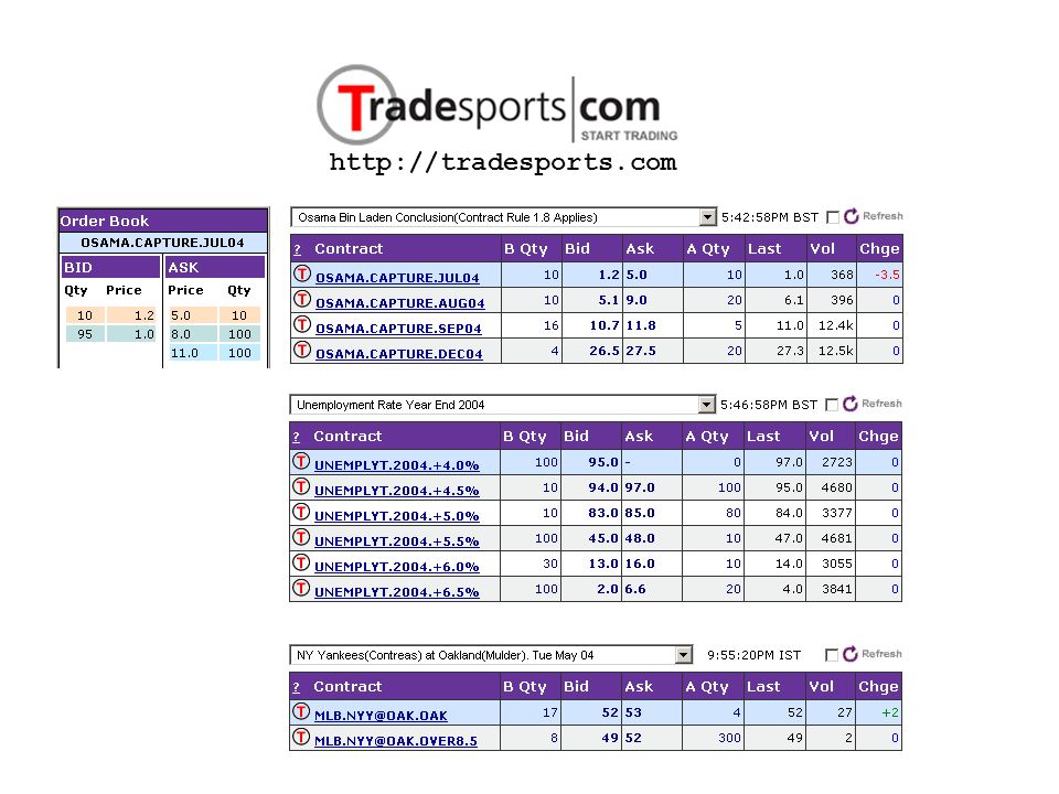


 for Microcontrollers>")

 Geometry (29%)>")


