1. Chapter 16: Correlation

2. So far… We’ve focused on hypothesis testing Is the relationship we observe between x and y in our sample true generally (i.e. for the population from which the sample came) Which answers the following question: Is there a relationship between x and y? (Yes or No) Where x is a categorical predictor and y is a continuous predictor

3. A new question… If there is a relationship between x and y… How strong is that relationship? How well can we predict a person’s y score if we know x? What is the strength of the relationship or the correlation between x and y

4. Memory Strategy Rote RehearsalSentenceInteractive Imagery Mean Recall

5. Memory Strategy Rote RehearsalSentenceInteractive Imagery Mean Recall                        

6. Memory Strategy Rote RehearsalSentenceInteractive Imagery Mean Recall                        

7. Memory Strategy Rote RehearsalSentenceInteractive Imagery Mean Recall                        

8. Memory Strategy Rote RehearsalSentenceInteractive Imagery Mean Recall

9. Memory Strategy Rote RehearsalSentenceInteractive Imagery Mean Recall 0 2 4 6 8 1010 1212 1414 1616 1818 2020 2 2424 2626                        

10. Memory Strategy Rote RehearsalSentenceInteractive Imagery Mean Recall 0 2 4 6 8 1010 1212 1414 1616 1818 2020 2 2424 2626                        

11. However… What if x is not a categorical variable What if x is a continuous predictor…e.g. arousal level And y is a continuous variable as well… e.g. performance level

12. Arousal Level LowMediumHigh Mean Performance Level 0 2 4 6 8 1010 1212 1414 1616 1818 2020 2 2424 2626

13. Arousal Level LowMediumHigh Mean Performance Level 0 2 4 6 8 1010 1212 1414 1616 1818 2020 2 2424 2626                        

14. Arousal Level LowMediumHigh Mean Performance Level 0 2 4 6 8 1010 1212 1414 1616 1818 2020 2 2424 2626                                                

15. Arousal Level LowMediumHigh Mean Performance Level 0 2 4 6 8 1010 1212 1414 1616 1818 2020 2 2424 2626                                                

16. Arousal Level LowMediumHigh Mean Performance Level 0 2 4 6 8 1010 1212 1414 1616 1818 2020 2 2424 2626                                                                                    

17. Arousal Level Mean Performance Level 0 2 4 6 8 1010 1212 1414 1616 1818 2020 2 2424 2626                                                                                    

18. Arousal Level Mean Performance Level 0 2 4 6 8 1010 1212 1414 1616 1818 2020 2 2424 2626                                                                                     02461010 1212 1414 1616 1818

19. Arousal Level Mean Performance Level 0 2 4 6 8 1010 1212 1414 1616 1818 2020 2 2424 2626                                                                                     02461010 1212 1414 1616 1818

20. The relationship between exam grade and time needed to complete the exam 100 90 80 70 60 50 40 20 3040506070 Grade (percent correct) Time to complete exam (in minutes)

21. Plots of values as a function of x and y PersonXY A11 B13 C32 D45 E64 F75 Y values 1 2 3 4 5 12345678 A B C D E F X values

22. 3 Characteristics of a Correlation: Direction of relationship Form of the relation Degree of the relationship

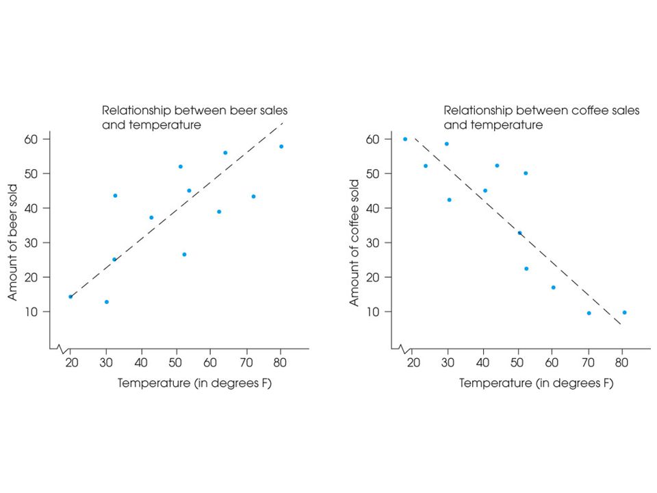
23. Correlations: Measuring and Describing Relationships (cont.) The direction of the relationship is measured by the sign of the correlation (+ or -). A positive correlation means that the two variables tend to change in the same direction; as one increases, the other also tends to increase. A negative correlation means that the two variables tend to change in opposite directions; as one increases, the other tends to decrease.

24. The relationship between coffee sales and temperature 60 50 40 30 20 3040506070 Amount of beer sold Temperature (in degrees F) 80 10

25. The relationship between beer sales and temperature 60 50 40 30 20 3040506070 Amount of coffee sold Temperature (in degrees F) 80 10

27. Correlations: Measuring and Describing Relationships (cont.) The most common form of relationship is a straight line or linear relationship which is measured by the Pearson correlation.

29. Comparison of performance based on amount of practice and male/female vocab scores 4 3 2 1 1234567 Amount of practice Performance (a) (b) Male Female Vocabulary score

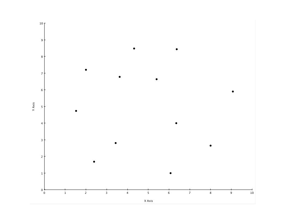
30. Correlations: Measuring and Describing Relationships (cont.) The degree of relationship (the strength or consistency of the relationship) is measured by the numerical value of the correlation. A value of 1.00 indicates a perfect relationship and a value of zero indicates no relationship.

31. Plot of points - wide dispersion 100 90 80 70 60 50 40 20 3040506070

32. Plot of points - narrow dispersion 100 90 80 70 60 50 40 20 3040506070

33. Examples of different values for linear correlations Y X (a) Y X (c) Y X (b) Y X (d)

34. Where and Why Correlations are Used: Prediction Validity Reliability Theory Verification

35. Correlations: Measuring and Describing Relationships (cont.) To compute a correlation you need two scores, X and Y, for each individual in the sample. The Pearson correlation requires that the scores be numerical values from an interval or ratio scale of measurement. Other correlational methods exist for other scales of measurement.

36. The Pearson Correlation The Pearson correlation measures the direction and degree of linear (straight line) relationship between two variables. To compute the Pearson correlation, you first measure the variability of X and Y scores separately by computing SS for the scores of each variable (SS X and SS Y ). Then, the covariability (tendency for X and Y to vary together) is measured by the sum of products (SP). The Pearson correlation is found by computing the ratio:

37. The Pearson Correlation (cont.) Thus the Pearson correlation is comparing the amount of covariability (variation from the relationship between X and Y) to the amount X and Y vary separately. The magnitude of the Pearson correlation ranges from 0 (indicating no linear relationship between X and Y) to 1.00 (indicating a perfect straight-line relationship between X and Y). The correlation can be either positive or negative depending on the direction of the relationship.

38. The Pearson Correlation

39. PDF version

40. Computational Examples

41. Computing the SP ScoresDeviationsProducts 13-2-2-2+4 26+1 44+1 57+2 +4 ( ) ( ) ( ) ( )

42. Understanding & Interpreting the Pearson Correlation Correlation is not causation Correlation greatly affected by the range of scores represented in the data One or two extreme data points (outliers) can dramatically affect the value of the correlation How accurately one variable predicts the other— the strength of a relation

43. The Spearman Correlation The Spearman correlation is used in two general situations: (1) It measures the relationship between two ordinal variables; that is, X and Y both consist of ranks. (2) It measures the consistency of direction of the relationship between two variables. In this case, the two variables must be converted to ranks before the Spearman correlation is computed.

44. The Spearman Correlation (cont.) The calculation of the Spearman correlation requires: 1. Two variables are observed for each individual. 2.The observations for each variable are rank ordered. Note that the X values and the Y values are ranked separately. 3.After the variables have been ranked, the Spearman correlation is computed by either: a. Using the Pearson formula with the ranked data. b. Using the special Spearman formula (assuming there are few, if any, tied ranks).

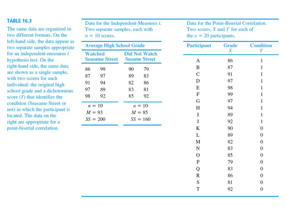
45. The Point-Biserial Correlation and the Phi Coefficient The Pearson correlation formula can also be used to measure the relationship between two variables when one or both of the variables is dichotomous. A dichotomous variable is one for which there are exactly two categories: for example, men/women or succeed/fail.

46. The Point-Biserial Correlation and the Phi Coefficient (cont.) In situations where one variable is dichotomous and the other consists of regular numerical scores (interval or ratio scale), the resulting correlation is called a point-biserial correlation. When both variables are dichotomous, the resulting correlation is called a phi-coefficient.

47. The Point-Biserial Correlation and the Phi Coefficient (cont.) The point-biserial correlation is closely related to the independent-measures t test introduced in Chapter 10. When the data consists of one dichotomous variable and one numerical variable, the dichotomous variable can also be used to separate the individuals into two groups. Then, it is possible to compute a sample mean for the numerical scores in each group.

48. The Point-Biserial Correlation and the Phi Coefficient (cont.) In this case, the independent-measures t test can be used to evaluate the mean difference between groups. If the effect size for the mean difference is measured by computing r 2 (the percentage of variance explained), the value of r 2 will be equal to the value obtained by squaring the point-biserial correlation.