1. Representation of spatial data
GIS thematic layers, raster and vector, conversion, subdivision representation, continuous data: contours, DEMs, TINs

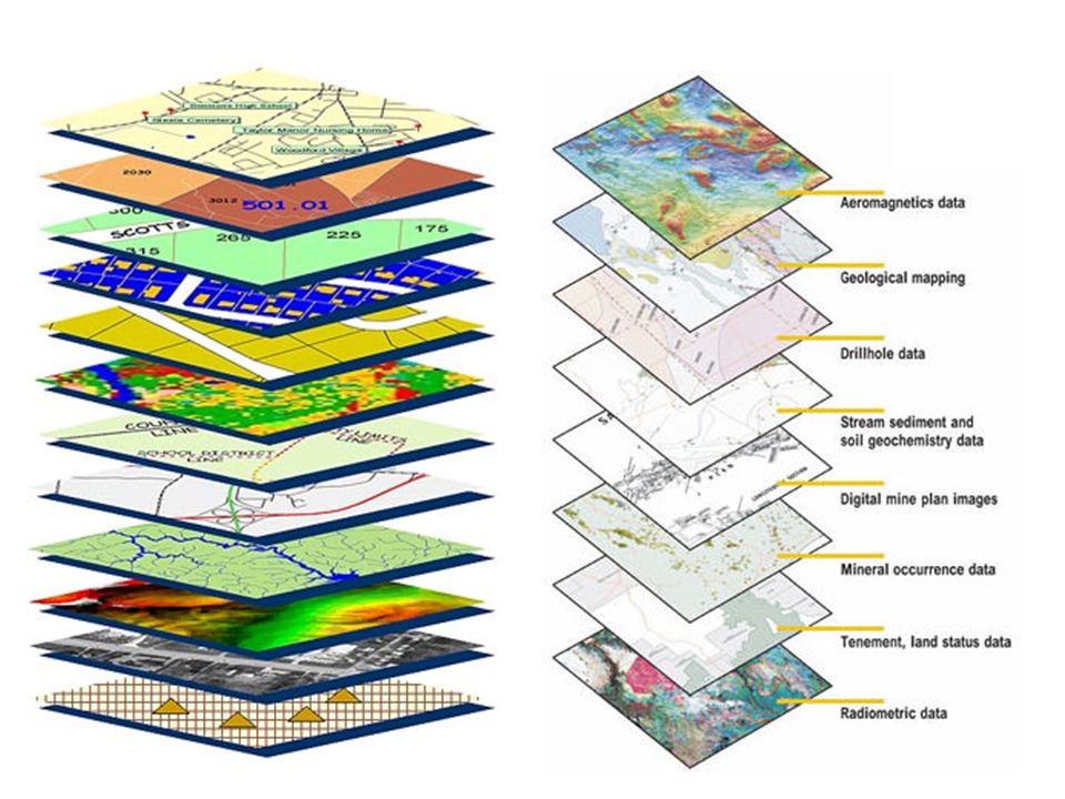
2. Thematic map layers
Separate storage of data according to theme: map layers (or data layers)
GIS typically use tens to hundreds of map layers
For example: municipality borders, land use, cadastral boundaries, water pipes, churches, etc.

4. Example map layers
Census data, 1995
(U.S.A.)

5. Geometry, topology and attributes
Geometry: coordinates
Topology: adjacency relations of objects
Attributes: properties, values
Example: Country map of South America
Geometry: coordinates of the borders Topology: which countries border which Attributes: names of countries, population, etc.

6. Representation of geometry
Two main approaches: raster and vector
Can also be mixed in a GIS, any map layer
Conversion raster-vector and vice versa possible
Representation depends on type of data, way of acquisition, desired operations, etc.

7. Raster structure
Division of space into equal-size cells (squares, pixels)
Theme gives cells a value (nominal, ordinal, interval, ratio, vector, …)
Cells should not contain any further spatial information (more detail)

8. Data in raster form Point object in raster form Line object in
Plane object in
raster form

9. Raster maps

10. Raster: pros and cons Simple structure Simple operations
Obtained after scanning, remote sensing
Less suitable for point and line objects: representation does not follow intuition
Network analysis difficult
Not adaptive: no difference in detail possible in different regions
Either expensive in memory, or little precision
Not obtained after digitizing

11. Raster: memory reduction
Run-length encoding: no 2-dim array but coding start pixel with value and length of run
Block encoding: 2-dim version
Disadvantage: makes structure and operations much more complex
(34,67) forest 9
(34,67) forest 4,6

12. Vector structure Objects stored as points, lines and areas
Points have coordinates; lines connect points; areas are delimited by lines
Attributes are stored with the objects (point, line or areal)

13. Vector: pros and cons
Elegant structure; fits with both point, line and areal objects
Small storage consumption
Precise
Adaptive: additional control points possible
Network and cluster analysis possible
Obtained after digitizing
Relatively complex
Map overlay and buffer computation complex

14. Vector representation of a region
Not necessarily simply-connected:
NL has islands
NL has holes (Baarle-Nassau / Baarle-Hertog); there are even regions in these holes

16. Representation of subdivisions

17. Subdivisions: spaghetti model
Every chain is represented by a list with coordinate pairs
Split nodes are doubly stored
Areas are not present explicitly C1 C2 C5 C4 C3 C6
C1: (..,..), (..,..), (..,..), ...
C2: (..,..), (..,..), (..,..), ...
C3: (..,..), (..,..), (..,..), ...

18. Subdivisions: polygon ring structure
Every area is represented by a list with coordinate pairs
Control points are doubly stored
Neighbor areas are difficult to determine
Consistency is difficult to maintain P1 P2
Consistency here refers to the property that a set of polygons should form a partition of a region. If you change the boundary of one polygon, you must change the boundaries of one or more other polygons as well to maintain the property that the polygons form a subdivision. Technically, consistency is not difficult to maintain, but it is an implementation hassle and causes inefficiency of updates, because these other polygons must be retrieved and changed as well. P3
P1: (..,..), (..,..), (..,..), ...
P2: (..,..), (..,..), (..,..), ...
P3: (..,..), (..,..), (..,..), ...

19. Subdivisions: topological structure (node-link structure)
Nodes are objects with coordinates
Edges are connections of nodes
Sequences of edges along polygon boundaries form cycles
Polygons are objects that can access their boundaries
Doubly-connected edge list

20. Subdivisions: topological structure
Edges are split into directed half-edges
Half-edges have pointers to
Twin half-edge
Origin vertex
Next and Prev half-edges of incident polygon
Incident polygon
Polygons have pointers to half-edges, one in each bounding cycle
Origin
polygon
Twin
Prev
Next
polygon

21. Subdivisions: topological chain structure
Splitting nodes are objects with coordinates
Chains are connections between splitting nodes and contain zero or more nodes with coordinates
Sequences of chains along polygon boundaries form cycles
Polygons are objects that can access their boundaries
half-chains
Doubly-connected chain list

22. Vector structures Memory Duplication Polygon Topology
retrieve retrieve
Spaghetti Polygon ring DC edge list DC chain list
Topology retrieve refers to the topology of the subdivision: region objects have a way to access adjacent regions efficiently. With a doubly-connected chain list, this comes down to following the chains and always looking at the other side of the chain for an adjacent region. This takes time linear in the number of adjacent regions, while for the doubly-connected edge list this takes time linear in the number of edges in the boundary of the region (which is much more). For the spaghetti and polygon ring structures, there is no easy access to adjacent regions and you have to traverse whole tables in the database.

23. Raster-vector conversion
E.g. for data integration
Vector-to-raster: Like in computer graphics: scan-conversion of lines, etc.
Raster-to-vector: Consider pixel sides between pixels with different values as boundary and put in vector representation  Thinning, line simplification

24. Thinning
Raster-vector
conversion
Thinning

25. Line simplification Douglas-Peucker algorithm from 1973
Input: chain p1, …, pn and error   p1 pn

26. DP-algorithm  Draw line segment between first and last point
If all points in between are within error: ready
Otherwise, determine farthest point and recursively continue on the part until farthest point and the part after farthest point

27. DP-algorithm DP-standard(i, j, )
Determine farthest point pk between pi and pj
If distance(pk, pi pj) >  then DP-standard(i, k, )
DP-standard(k, j, )
Return the concatenation of
the simplifications

28.   

29.   

30. Properties of the DP-algorithm
DP-algorithm does not minimize the number of points in the simplification   
DP-algorithm
Optimal

31. Properties of the DP-algorithm
Determining farthest point takes O(n) time
Whole algorithm takes T(n) = T(m) + T(n-m+1) + O(n), T(2) = O(1) time, splitting in m and n-m+1 points
“Fair” split gives O(n log n) time
Worst case gives quadratic time

32. Properties of the DP-algorithm
DP-algorithm may give self-intersections in the output 
Solution: test output for self-intersections and continue adding control points if necessary

33. Improved DP-algorithm
DP-improved(i, j, )
Simp = DP-standard(i, j, )
V = set of intersecting segments of Simp Repeat
For all segments s  V: Refine(s) in Simp; do 1 refinement à la DP by adding the farthest point, giving a new Simp V = set of intersecting segments of Simp Until V is empty

34. Continuous data representation
Digital Elevation Model (DEM)
Data on interval or ratio measurement scale
Data values of points near by will usually be not very different
Representation is necessarily an approximation: finite representation of information with infinite detail
Raster (1x) or vector (2x)

35. Elevation models Raster Vector Vector (Elevation) grid21 20 21 20 15 20 19 25 10 10
(Elevation) grid
Contour line model
Triangulation (TIN; triangulated irregular network)

36. Grid elevation model

37. TIN elevation model

38. Elevation models
Contour model well-suited for visualisation, not for representation or storage
Interpretations grid: - elevation whole cel: not a continuous model - elevation middle cel: interpolation needed; how?
Advantage grid: simple storage, operations simple too
Advantage TIN: more efficient in storage, adaptive

39. Interpolation for grid20 18 20 18 18 22 18 22 20 18
Linear interpolation; saddle point problem 18 22 20 18 20 18 18 22 18 22
Linear interpolation; additional point 4
= 19.5
Non-linear
interpolation

40. Topological TIN structure
With explicit vertex and triangle representation t2 w t3 t1 t1 t2 t t u v u w t3 v
x, y-coordinates and elevation

41. Topological TIN structure
With explicit vertex and triangle representation t2 w t3 t1 t1 t2 t t u v u w t3 v
Because t1 has pointers to two the same vertices as t, we can determine their shared edge, even though it is not represented explicitly

42. Topological TIN structure
With explicit vertex and triangle representation w w t1 t2 t2 t1 t u v t t3 v u t3

43. Topological TIN structure
Alternatively, edges have an explicit representation too w t1 t2 w t1 t e1 e2 e1 e2 u e3 v t3 t u v e3

44. Summary representation
Objects have geometry and attributes, at least the attributes are in a database
Geometry can be stored in raster or vector form; each has advantages and disadvantages
Important geometric types of representations are those for subdivisions and for elevation models
For subdivisions, the doubly-connected chain list is the most suitable structure
For elevation models, grids or TINs are most useful