1. Diagnostics and Instrumentation for ERL  Pieces of ERL and their beam specifics  Injector diagnostics  Drive Laser diagnostics  Problems with 2-beam Linac  Large dynamic range measurements – direction of development  Transversal beam match  Longitudinal match, bunch compression, bunch length measurements Pavel Evtushenko, JLab

2. ERL regions and their specific 1.Electron gun / injector: low 5-10 MeV beam energy space charge dominated beam transversely large, few ps long 2. Linac: two beams, must preserve beam quality 7. Beam dump put all in there 3. Beam transport: higher beam energy, bunch compression, match transversely 4. FEL wiggler (interaction region) transversely smallest beam, shortest bunch length, precisely set Twiss parameters, no beam loss, precise trajectory to overlap with optical mode 5. More beam transport the same, but used beam 6. More Linac used beam, energy compression 0. Drive Laser / Photocathode: change and affect everything

3. Gun / Injector diagnostics Beam parameters that need to be measured and monitored in the injector:  the transverse phase space distribution (Twiss parameters and emittance )  the longitudinal phase space distribution (bunch length and energy spread)  be able to measure and control halo  phase of the beam in RF cavities (1. setup 2. monitor)  drive laser parameters (transverse & longitudinal profile, position, phase )  cathode (Q.E.) distribution  make sure that the beam parameters measured with tune-up pulsed beam do not change when going to CW beams and changing the beam average current

4. Gun / Injector diagnostics Viewers (3) Solenoids (2) Quads (4) SRF cavities (2)Electron gun (1)

5. Injector / Transverse beam profile  100 um thin YAG:Ce viewers oriented normal to the beam is used  first viewer (on the left) located downstream of the booster in non dispersive location  used when centering beam in injector elements, emittance measurements and beam phase  second viewer (on the right) located at the point close to max. dispersion and small horizontal beta function  used for energy spread (energy distribution) and mean energy measurements also beam phase

6. Injector / Transverse Phase Space The multislit or a single slit scanning through the beam (or a beam scanning across the slit) does the job very well (pulsed beam only).  well established technique  works for space charge dominated beam  beam profile is measured with YAG  measures not only the emittance but the Twiss parameters as well  enough information to reconstruct the phase space  has been implemented as on-line diagnostics  works with diagnostics mode only (low duty cycle, average current)

7. Injector / Longitudinal Phase Space  Single cell cavity or multi-cell structure with TM dipole mode impose on the bunch time dependent transverse kick.  The dipole creates dispersion in the transverse direction perpendicular to the cavity kick Problems:  the same as multislit – pulsed beam only  resolution limited by transverse emittance; solution – put a small hole in front of the cavity and do the measurements for small beamlet AND as f(x,y) - 3D charge distribution  usually a special setup placed at the beam line for injector study and removed when it is done.

8. Injector / Drive Laser Diagnostics  Transversal profile of the D.L. on the cathode (standard technique) imaging reflection from the input window to a CCD placed on the same distance from the window as the cathode  Longitudinal profile: auto-correlator works well for Gaussian pulses for non Gaussian pulses streak camera  Amplitude stability photo diode (at JLab FEL is monitored all the time in control room)  Transversal stability long term slow drifts or misalignment – the same CCD as for profile meas. fast transverse jitter 4-quadrant position sensitive photodiode  Phase stability (phase noise) all the way down to DC fast (few GHz) photodiode to look at FM at very high harmonic number BUT also must do measurements at DC to separate AM from FM + Signal Source Analyzer (SSA) expansive but saves a lots of time

9. Injector / Drive Laser Diagnostics  all focusing elements are placed upstream of the pick off plate  distance from the pick off to the cathode = distance from pick off to reference screen  the reference screen used for D.L. profile and position measurements

10. Injector / Drive Laser Diagnostics Typical auto-correlator signal JLab FEL D.L. (observed in the control room permanently) Drive Laser transverse profile dynamic range ~500: 10-bit frame grabber, 60 dB SNR CCD

11. Injector / Cathode Q.E.  For accurate modeling of the injector beam dynamics the input in to a code must be accurate. This includes the emission transversal profile, which is a product of the Drive Laser profile and Q.E. profile  One technique to measure the Q.E. profile is scanner with a laser (spot on the cathode is much smaller than cathode dimensions) and two scanning mirrors. Usually automated and gives 2D distribution of the Q.E. Can be used only with beam and gun voltage off.  Another technique: run low current emittance dominated beam (even DC), measure the laser trans. profile and image the cathode to a view screen. The ration of the beam profile and the laser profile gives Q.E. profile. If used with the real drive laser (not always possible) gives the emission profile. Laser profile on cathodePhotoemission profile

12. 2-pass viewers  there are two beams in the LINAC  when trying to measure decelerating beam with a viewer the accelerating beam gets also intercepted  ultimately the measurements should be done with non intercepting technique (or intercepting but negligibly )  JLab FEL uses OTR viewers with 5 mm hole (first beam goes in to the hole)  44% transparent mesh 5 micron thin  SRF cavities see the radiation due to the intercepted beam (can trip cavity) JLab FEL LINAC OTR viewer  With the ultra bright beam OTR might be useless (OTR  COTR like @ LCLS)  The best solution might be to use wire scanners (intercepts small part of the beam).  If the scanner measures radiation created by the wire, must take care of the background.  Laser wire scanner: Will the measurements time and cost be acceptable? What is the lowest energy when the technique is practical?  We also use: 1. Diamond-like carbon foils ~ 1 micron thin

13. 2-pass BPM (ideas) Stripline BPM signal measured with scope, the picture limited by the scope BW  A. Lebedev proposed at ERL05 to make a system based on small AM of the beam current (no experiments so far)  Time domain approach might be very different for different machines ✔ long recirculation time vs. short; ✔ every bucket filled vs. not  The phase difference is not always 180 deg, especially when tuning machine  In JLab FEL the ΔT between two beam depends on rep. rate.; smallest is 6 ns; Time domain approach: (will not measure every bunch) 1. make BPM pulses broader to 1.5 ns (LPF or dispersion) 2. grab peak value with S&H (GHz BW) 3. digitize S&H output with ~ 10 MHz ADC Motivation:  To do differential orbit measurements (measure transport matrix) with both beams in the LINAC  The decelerating beam gets adiabatically anti-dumped – small errors corrections in the beginning leads to big orbit change at the end  Orbit stabilization and feedback

14. Transport / Transverse match  combination of OTR and P-46 phosphor coated viewer is used  set of transverse beam profiles measured through UV FEL beam line (~1/2 of the accelerator)  together with the machine optics model used to understand and adjust the transverse match  iterative process between measurements and fitting/adjusting model and beam optics  anything but Gaussian distributions

15. Large dynamic range beam profile measurements Measured in JLab FEL injector, local intensity difference of the core and halo is about 300. (500 would measure as well) 10-bit frame grabber & a CCD with 57 dB dynamic range PARMELA simulations of the same setup with 3e5 particles: X and Y phase spaces, beam profile and its projection show the halo around the core of about 3e-3. Even in idealized system (simulation) beam dynamics can lead to formation of halo.

16. Large dynamic range measurements (example)  Main principal of one of the ways to make large dynamic range measurements is to reduce a measurement to frequency measurements. Then make it work for 1 Hz and for 100 MHz and this is 10 8 dynamic range.  For instance use PMT and keep them working in counting mode.  Can be applied to e - beam measurements, laser, (light), X-rays.  Example: wire scanner measurements: Courtesy of A. Freyberger (measured at CEBAF)

17. Drive Laser large dynamic range measurements  typically in simulation the drive laser pulse is assumed “ideal” i.e. as we want it  to find out how far is it true and if concerned about 1e-6 details of the phase distribution there is the need to make D.L. pulse measurements with 1e6 dynamic range  transverse and longitudinal profile of the D.L. needs to be measured  AND reflections from D.L. transport, which might be far from D.L. spot (also in time)  for transversal profile measurements: ➟ could use 120 dB dynamic range CCD (2 CCD in one camera each 60 dB) ➟ use a usual ~ 60 dB CCD with an ND filter and accurate cross-calibration  for longitudinal profile measurements: ➟ auto-correlator with dynamic range 120 dB can be built using PMT ➟ auto-correlator works fine for Gaussian pulses ➟ WHAT to do for non Gaussian?

18. Drive Laser “ghost” pulses  For machine tune up, beam studies, intercepting diagnostics a “diagnostic beam” with very low average current but nominal bunch charge is used (all beam can be lost without damaging machine)  For example, JLab FEL: max rep. rate 74.85 MHz (CW) diagnostic mode: rep. rate 4.678125 MHz (÷16), 250 μs / 2 Hz (÷2000) average current ~300 nA  Most of the laser pulses are “stopped” by EO cell(s), but the extinction ratio of the an EO cell is about 200 (typical), two in series ~ 4×10 4  Another example: want to reduce 1300 MHz (100 mA) to 300 nA (2 18 ) than for every bunch Q b we want we also get 6.55×Q b of “ghost” pulses (655 % !!!) we do not want  “ghost” pulses overall intensity must be kept much lower than real pulses!!! for “usual” measurements ~ 1% might be fine much bigger problem if want to study halo, let’s say 10 -6 effects, than “ghost” pulses should be kept at 10 -8 (???)

19. Drive Laser “ghost” pulses  Using a Log-amp is an easy way to diagnose presence of the “ghost” pulses Beam current measurements with a linear circuit current measurements with A Log-amp circuit (60 dB) Problem:  this does not work for CW beam

20. Drive Laser “ghost” pulses  Using a Log-amp is an easy way to diagnose presence of the “ghost” pulses  Log-amps with dynamic range 100 dB are available 631 uA (100%) 135 pC x 4.678125 MHz 5.7 uA (~0.9 %) 37.425 MHz “ghost” pulses

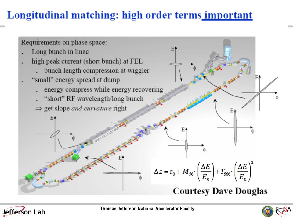
22. Longitudinal transfer function measurements The M 56 and T 566 transport matrix elements are validated via longitudinal transfer function measurements – essential for optimal bunch compression. T 566 is adjusted by sextupoles in dispersive location (ARC1) M 56 is adjusted by quadrupoles in dispersive location (ARC1) Changes in the E 0 and it effect on the bunch compression

23. Pulsed and CW beam measurements / transition  Most affordable way to measure ps and sub-ps bunches  Works with pulsed beam (tune up) and CW beam, essentially at any average current  Used at JLab FEL to ensure that the bunch length does not change for pulsed or CW and when the average current is increased  Ultimately needs to be setup in vacuum (or N 2 purge) due to atmosphere absorption of THz  Phase information is lost – no direct bunch profile reconstruction  A detector measuring total CTR (CSR) power – a bunch length monitor Power spectrum Interferogram (autocorrelation)

24. Conclusion and Outlook  Most of the measurements can be made with fairly simple diagnostic tools  For an injector transverse and longitudinal phase spaces can be measured very well with pulsed (diagnostics) beams.  One direction to improve that is to increase the dynamic range of such measurements to (10 6 – 10 8 ?)  Another direction of improvement and development is to monitor injector beam parameters with CW beam (beam size most challenging)  Measurements of D.L. with big dynamic range to understand beam dynamics with the same big dynamic range  LINAC (part of the machine with 2 beams) needs specific solutions  reducing the CW beam to diagnostic beam needs careful consideration this (via “ghost” pulses) affects all diagnostics

25. Conclusion and Outlook (2)