1. Where is calibration (S o )for aerosol optical depth measurements? Or Practical sun spectral radiometer calibration methods. Or Learning from mistakes!

2. History Indicates ‘The three most important issues in sun photometry are: calibration; calibration; and calibration.’ Michalsky (2000)

3. Experience Suggests Mauna Loa’s don’t exist except at Mauna Loa! Subjective estimates of determining what is a valid ‘Langley’ are dubious. Sites with low incidence of extended clear sun periods have a low chance of success with atmospheric methods. Quantitative filters are better than qualitative filters.

4. Why is the calibration of sun spectral radiometers so difficult? There is no WRR and absolute spectral radiometers in field use! We are mainly interested in a derived quantity (aerosol optical depth) that requires more precision than irradiance measurement. Lack of stable detector-based reference. The stability of the commonly used filter radiometers is poor. We need to have reference of spectral irradiance AND the irradiance at the top of the atmosphere.

5. Spectral Irradiance Signal Equation S (t) = (r 0 /r) 2 S 0 exp(-  m i (t)  i (t)) + F(t,S,  ) S (t) = signal measured at time t at wavelength S 0 = signal at the top of the atmosphere at 1 AU F(t,S,  ) = circumsolar contribution to the signal  m i (t)  i (t) = extinction components (molecular, aerosol, ozone,…) (r 0 /r) 2 =earth sun distance correction for S 0

6. Short cuts to avoid my mistakes: Atmospheric methods For properly designed instruments we can reduce the uncertainty in the measured sun signal. If  is the small F() can be ignored. In molecular, aerosol, ozone-only regions of the spectrum and  < 10 nm the Bouguer-Beer-Lambert ‘law’ may apply; hence ln S (t) = 2 ln(r 0 /r) + ln S 0 -m m (t)  m (t) -m a (t)  a (t) -m o (t)  o (t) Then can use Least Squares Regression to estimate ln S 0.

7. Least squares regression (LSQ) For a set of n pairs of (x,y) observations where we assume the relationship is y(t) = A x(t) + B The LSQ allows us to estimate A and B by = [  (x(t) – X)(y(t)- Y)]/[  (x(t)-X) 2 ] = Y - X where X and Y are the mean values.

8. Other LSQ parameters  2 = [  (y(t) - x(t) - ) 2 ]/[n – 2] = variance of the estimate in y(t)  = standard error of the estimate in y(t) S x = [  (x(t) – X) 2 ]/[n-1] S y = [  (y(t) – Y) 2 ]/[n-1] r = S x / S y = correlation coefficient, with r 2 = coefficient of determination

9. Atmospheric methods The atmospheric methods assume that a simple linear expression y(t) = A x(t) + B of known variables x and y for a period of times t is a valid model of how the atmosphere is interacting with the radiation extinction. Most importantly use of LSQ for determining the calibration S o assumes that the variation of A and/or B is randomly and normally distributed about the model. Given that the atmosphere is rarely static and rather dynamic it is important to select x and y terms that ensure that A and B have little potential variation and uncertainty.

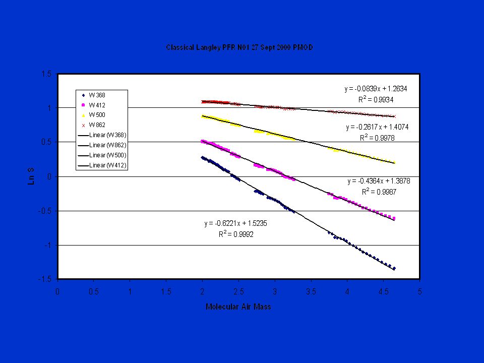
10. Classical ‘Langley’ m m  =   i m i F() = 0.0 Using x(t) = m m (t) y(t) = ln S (t) and derive = = + 2 ln(r 0 /r) The classical model assumes that variation in  is very small over t hence it is essential to restrict the period of observations to very clear sun periods where the  m m /  t is high but there is little uncertainty in the signal; usually between m m = (2.0, 6.0). Also need to know m m (t).

13. Modified ‘Langley’ x(t) = m a (t) y(t) = ln S (t) + m o (t)  o (t) + m m (t)  m (t) and derive = and = + 2 ln(r 0 /r) The modified model assumes that variation in  a is very small over the measurement period: restrict the period of observations to very clear sun periods where the  m m /  t is high but there is little uncertainty in the signal; usually between m a = (2.0, 6.0). Also need to know m o (t),  o (t), m m (t), and  m (t).

17. Other information on the Classical and Modified ‘Langley’ These methods explicitly give more weight to periods of high airmass because they are minimizing (ln S (t) - 2 ln(r 0 /r) + - m (t) ) 2 and not the variance in optical depth  which is the parameter one expects to be varying randomly and having a normal distribution through the period of observation.

18. Unweighted ‘Langley’ x(t) =1/m a (t) y(t) = (ln S (t) + m o (t)  o (t) + m m (t)  m (t))/m a and derive = + 2 ln(r 0 /r) and = In this case the minimization is of  a, however it does assume that variation in  a is very small over the measurement period hence it is essential to restrict the period of observations to very clear sun periods where the  m m /  t is high but there is little uncertainty in the signal; usually between m a = (2.0, 6.0). Also need to know m o (t),  o (t), m m (t), and  m (t).

20. Varying aerosol conditions All the previous methods assume that there are no trends in the optical depth components over the range of airmass, particularly  a. The next methods remove the restriction on a ‘constant’ optical depth, and utilise the interaction between aerosols and radiative propagation. We know that most natural aerosol size distributions will produce a smoothly variation of aerosol optical depth with wavelength. Furthermore, if the relative size distribution of the aerosols remains the same the aerosol optical depth is directly proportional to the total number of particles. e.g.  a ( ) =  ( /1000) - 

21. Aerosol optical depth  a ( ) = c  Q ex (x) (dn/dln r) dln r where x = 2  r/, Q ex is the extinction efficiency (that is dependent on the complex refractive index of the aerosol) and dn/dln r is the aerosol number density

22. Aerosol optical depth a function of Under most circumstances a single aerosol set of aerosol properties influences the extinction across wavelength. It is also known that the most optically active aerosols (r = 0.2  1.0  m) are those with the longest lifetime. It is clear that there is good correlation between  a ( 1 ) and  a ( 2 ) and any change in the natural aerosol distribution will impact on most wavelengths (0.3 – 3 µm).

23. Relational methods These methods require the calibration of one wavelength channel to be known, and then in various conditions the signals from that channels can be related to other channels. Two useful methods are: (1) ratio-Langley and (2) general method

24. Ratio-Langley method x(t) =m m (t) y(t) = (ln S 1 (t)/ S r (t) and derive = = It is easy to show that the variability in (  1 -  r ) is much less than the variability in either  1 or  r in periods of moderately varying aerosol optical depth and the uncertainty deceases as 1  r. This method is particularly useful when comparing similar nominal wavelengths with the resultant indicating minor differences between 1 and r. (This method is not new – it is the primary method used in Dobson Spectrometers for deriving calibration and ozone parameters).

25. General method This method uses the ‘aerosol optical depth’ derived from a well-calibrated channel (or in some cases the aureole derived aerosol extinction). For a well calibrated channel we can derive the aerosol component of extinction at r as -m a (t)  ar (t) = ln S r (t) +m m (t)  mr (t) +m o (t)  or (t) -2 ln(r 0 /r) - ln S 0r x(t) = - m a (t)  ar (t), y(t) = ln S (t) + m o (t)  o (t) + m m (t)  m (t) and derive = and = + 2 ln(r 0 /r) The general model assumes that variation in the relative aerosol optical depths (  a /  ar )is very small over the measurement period, even if there are moderate variations in the absolute magnitude. Like the other methods the period of observations is restricted to clear sun periods where the  m m /  t is high but there is little uncertainty in the signal; usually between m a = (2.0, 6.0). Also need to know m o (t),  o (t), m m (t), and  m (t) for both the reference and calibrated channels.

27. Summary PFR N01 27 Sept 2000 Davos Method368 nm412 nm500 nm862 nm Classic0.1240.1060.0850.054 Modified0.1130.09700.0870.050 Un-Weighted0.1280.1090.0950.055 Ratio-Langley0.0167(0.018)-0.022-0.025 General0.0016(-0.002)0.00110.0105

28. Checks and Balances It is important to realise that no single calibration derived from any of these calibration methods at typical sites will produce a useful value! Only by multiple calibrations typically over a month or two with at least 20 good points will a valid calibration be produced.

30. Single wavelength methods Methodx(t)y(t) Gradient Intercept Classic Langley m m (t)ln S (t)  ln S 0 + 2 ln(r 0 /r) Modified Langley m a (t)ln S (t) + m o (t)  o (t) + m m (t)  m (t) aa ln S 0 + 2 ln(r 0 /r) Weighted Langley 1/m a (ln S (t) + m o (t)  o (t) + m m (t)  m (t)) /m a ln S 0 aa

31. Relational methods Methodx(t)y(t) Gradient Intercept Ratio- Langley m m (t) ln (S (t)/S r (t))  -  a r ln (S 0 /S 0r ) General- m a (t)  ar (t) ln S (t) + m o (t)  o (t) + m m (t)  m (t)  a /  ar ln S 0 + 2 ln(r 0 /r)

32. Quotes to Remember ‘The accuracy of results is inversely proportional to the promptness of publication’ Robinson (1970) ‘Science is the search for ignorance’, Feynman (1963)

33. So what men knew about seasons was true and sometimes not; it was questionable but not knowable, discernible by its origins but obscure in its presence and in its moment of ending. It was like so many things men accepted without wonder. Yet in that uncertainty lay the pivot point of existence. Fortress of Eagles C J Cherryh