1. Cervical Cancer Case Study Presented by: University of Guelph Baktiar Hasan Mark Kane Melanie Laframboise Michael Maschio Andy Quigley

2. Objectives To determine an appropriate model for the prediction of recurrence of cervical cancer To classify future patients on their risk of recurrence of cervical cancer

3. Cervical Cancer Data Set The original data set included 905 cases Patients were removed from the data set if they had ANY of the following: Were NOT free of the disease after surgery  845 Cases remain NO follow up date ZERO survival time

4. Modeling Methods Mixture Model with Accelerated Failure time –Peng and Debham (1998) Cox Proportional Hazard Model Latent Variable Model Bayesian Survival Analysis –Seltman, Greenhouse, and Wassserman (2001) –Chen, Ibrahim, and Sinha (1999)

5. Mixture model The model we chose for modeling time to recurrence is a mixture model of the form: S(t)=pS u (t) + (1-p) F(t)=pF u (t) Benefits: Allows for cure rate Covariates can be incorporated into survival time [S u (t)] AND\OR cure rate [1-p]

6. Mixture Model (Con’t) The model can be fit using a S-plus library (GFCURE) written by Peng. Further details about the library and the model can be found in Peng et al. (1998) and Maller and Zhou (1996). It should be mentioned that we found an error in the S-plus library written by Peng. The function pred.gfcure has a small error which can cause the program to crash or produce incorrect predicted values in some situations.

7. “Immunes” and Sufficient Follow up Maller and Zhou (1996) suggest tests to examine the hypotheses of: –Presence of “immunes” in the data set –Sufficient follow up time In the data set, it was found that immunes were present and there was not strong evidence to suggest that follow up time was insufficient

8. Missing Covariates It was noticed that a large proportion of the cases (≈40%) had at least one covariate with a missing value Various methods to handle this situation include: –Ignoring cases with missing covariate data –Maximum Likelihood Methods Chen and Ibrahim (2001)

9. Missing Covariates (Con’t) We chose to perform variable selection on only the cases that contain no missing covariates (n=534). BIAS introduced ??? CHECK: compare distributions of covariates in “full” and “reduced” data sets NO significant bias was introduced

10. Distribution A variety of distributions were considered for modeling recurrence time including Weibull, gamma, lognormal, log- logistic, extended generalized gamma and generalized F. From comparing the distributions using AIC for the above models, there was little improvement from fitting a distribution with 3 or 4 parameters versus a 2 parameter distribution. Of the 2 parameter distributions considered the Weibull distribution surfaced as the best distribution in terms of likelihood and prediction of the cure rate.

11. Variable Selection Stepwise variable selection was performed using the 534 patients previously mentioned; AIC was used as the entering criterion. Variables were allowed to enter both the cure rate portion of the model and survival time portion of the model. The final model chosen uses the explanatory variables pelvis lymph node involvement (PELLYMPH) and size of tumor (SIZE) to model the survival time of uncured patients and uses Capillary Lymphatic Spaces (CLS) and depth of tumor (MAXDEPTH) to predict cure rate.

12. Variable Selection (Con’t) It should be noted that CLS was modeled as a continuous variable rather than discrete because twice the difference of log likelihoods from modeling CLS as continuous versus discrete is 0.017. Interactions of the significant covariates in the chosen model were also considered, but were found to be non-significant.

13. Chosen Model VariableCoefficientS.E.p-value Terms in accelerated failure time model PELLYMPH-1.07270.36760.0035 SIZE-0.05780.0111<0.0001 Terms in the logistic model CLS0.92030.29880.0021 MAXDEPTH0.05610.02060.0081

14. Interpretation of the Model The negative coefficient of PELLYMPH indicates that uncured patients found positive for pelvis lymph node involvement will have a lower recurrence time than patients found negative for pelvis lymph node involvement. The coefficient of SIZE is also negative, which means that for uncured patients, larger tumor size corresponds to quicker recurrence of cancer. The positive value of CLS in the cure rate portion of the model indicates that patients with a positive prognosis have a higher probability of recurrence. The coefficient of MAXDEPTH is also positive, indicating that patients with a large tumor depth have a higher probability of recurrence.

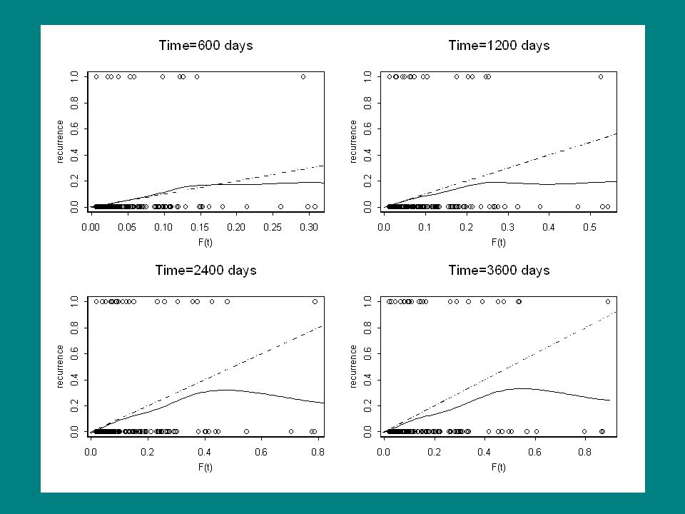
15. Model Validation In order to determine how well the chosen model will predict future patients, the data was randomly split into two subsets. Since it is not known if a patient who did not relapse was cured or censored it is not possible to compare the predicted probability of recurrence with the actual probability of recurrence. A graphical method was utilized for determining how well the predicted probabilities performed.

16. Model Validation (Con’t) The graphical method involved predicting the probability of recurrence before time t i (F(t)) for a number of chosen times. This prediction is smoothed against recurrence, which is 1 if recurrence occurred before time t i or 0 if recurrence has not occurred before time t i A criticism of this graphical method is that it is possible for a patient with a survival time less than t i but no recurrence to have a recurrence between their censored survival time and t i so they should have been coded as a 1 not a zero for the graph.

18. Classification The second objective is to classify patients into 3 groups: Low relapse, Moderate relapse, and High relapse. We classified patients based on their estimated cure rate from the final model previously mentioned. Low relapse: estimated cure rate ≥ 94% Moderate relapse: 84% < estimated cure rate < 94% High relapse: estimated cure rate ≤ 84%

20. Conclusions We found that the attributes Capillary Lymphatic Spaces and depth of tumor are important for predicting the probability of relapse and pelvis lymph node involvement and size of tumor are important for predicting the survival time of uncured patients. We used these attributes in a Weibull mixture model to classify patients according to their risk of recurrence.

22. References Chen, M., and Ibrahim, J. (2001), “Maximum likelihood methods for cure rate models with missing covariates” Biometrics, 57, 43-52. Chen, M., Ibrahim, J., and Sinha, D. (1999), “A new bayesian model for survival data with a surviving fraction” JASA, 94, 909-919. Maller, R., and Zhou, X. (1996), Survival Analysis with Long-Term Survivors. Toronto: John Wiley & Sons. Peng, Y., Dear, K., and Debham, J. (1998), “A generalized F mixture model for cure rate estimation” Statistics in Medicine, 17, 813-830. Seltman, H., Greenhouse, J., and Wasserman, L. (2001), “Bayesian model selection: analysis of a survival model with a surviving function” Statistics in Medicine 20, 1681-1691.