1. Artificial Neural Networks 1 Morten Nielsen Department of Systems Biology, DTU IIB-INTECH, UNSAM, Argentina

2. InputNeural networkOutput Neural network: is a black box that no one can understand over-predicts performance Overfitting - many thousand parameters fitted on few data Objectives

5. Weight matrices (PSSM) A weight matrix is given as W ij = log(p ij /q j ) –where i is a position in the motif, and j an amino acid. q j is the background frequency for amino acid j. W is a L x 20 matrix, L is motif length A R N D C Q E G H I L K M F P S T W Y V 1 0.6 0.4 -3.5 -2.4 -0.4 -1.9 -2.7 0.3 -1.1 1.0 0.3 0.0 1.4 1.2 -2.7 1.4 -1.2 -2.0 1.1 0.7 2 -1.6 -6.6 -6.5 -5.4 -2.5 -4.0 -4.7 -3.7 -6.3 1.0 5.1 -3.7 3.1 -4.2 -4.3 -4.2 -0.2 -5.9 -3.8 0.4 3 0.2 -1.3 0.1 1.5 0.0 -1.8 -3.3 0.4 0.5 -1.0 0.3 -2.5 1.2 1.0 -0.1 -0.3 -0.5 3.4 1.6 0.0 4 -0.1 -0.1 -2.0 2.0 -1.6 0.5 0.8 2.0 -3.3 0.1 -1.7 -1.0 -2.2 -1.6 1.7 -0.6 -0.2 1.3 -6.8 -0.7 5 -1.6 -0.1 0.1 -2.2 -1.2 0.4 -0.5 1.9 1.2 -2.2 -0.5 -1.3 -2.2 1.7 1.2 -2.5 -0.1 1.7 1.5 1.0 6 -0.7 -1.4 -1.0 -2.3 1.1 -1.3 -1.4 -0.2 -1.0 1.8 0.8 -1.9 0.2 1.0 -0.4 -0.6 0.4 -0.5 -0.0 2.1 7 1.1 -3.8 -0.2 -1.3 1.3 -0.3 -1.3 -1.4 2.1 0.6 0.7 -5.0 1.1 0.9 1.3 -0.5 -0.9 2.9 -0.4 0.5 8 -2.2 1.0 -0.8 -2.9 -1.4 0.4 0.1 -0.4 0.2 -0.0 1.1 -0.5 -0.5 0.7 -0.3 0.8 0.8 -0.7 1.3 -1.1 9 -0.2 -3.5 -6.1 -4.5 0.7 -0.8 -2.5 -4.0 -2.6 0.9 2.8 -3.0 -1.8 -1.4 -6.2 -1.9 -1.6 -4.9 -1.6 4.5 SLLPAIVEL YLIPAIVHI TLWVDPYEV

6. Biological Neural network

7. Biological neuron structure

9. Transfer of biological principles to artificial neural network algorithms Non-linear relation between input and output Massively parallel information processing Data-driven construction of algorithms Ability to generalize to new data items

11. Similar to SMM, except for delta function!

14. How to predict The effect on the binding affinity of having a given amino acid at one position can be influenced by the amino acids at other positions in the peptide (sequence correlations). –Two adjacent amino acids may for example compete for the space in a pocket in the MHC molecule. Artificial neural networks (ANN) are ideally suited to take such correlations into account

15. SLLPAIVEL YLLPAIVHI TLWVDPYEV GLVPFLVSV KLLEPVLLL LLDVPTAAV LLDVPTAAV LLDVPTAAV LLDVPTAAV VLFRGGPRG MVDGTLLLL YMNGTMSQV MLLSVPLLL SLLGLLVEV ALLPPINIL TLIKIQHTL HLIDYLVTS ILAPPVVKL ALFPQLVIL GILGFVFTL STNRQSGRQ GLDVLTAKV RILGAVAKV QVCERIPTI ILFGHENRV ILMEHIHKL ILDQKINEV SLAGGIIGV LLIENVASL FLLWATAEA SLPDFGISY KKREEAPSL LERPGGNEI ALSNLEVKL ALNELLQHV DLERKVESL FLGENISNF ALSDHHIYL GLSEFTEYL STAPPAHGV PLDGEYFTL GVLVGVALI RTLDKVLEV HLSTAFARV RLDSYVRSL YMNGTMSQV GILGFVFTL ILKEPVHGV ILGFVFTLT LLFGYPVYV GLSPTVWLS WLSLLVPFV FLPSDFFPS CLGGLLTMV FIAGNSAYE KLGEFYNQM KLVALGINA DLMGYIPLV RLVTLKDIV MLLAVLYCL AAGIGILTV YLEPGPVTA LLDGTATLR ITDQVPFSV KTWGQYWQV TITDQVPFS AFHHVAREL YLNKIQNSL MMRKLAILS AIMDKNIIL IMDKNIILK SMVGNWAKV SLLAPGAKQ KIFGSLAFL ELVSEFSRM KLTPLCVTL VLYRYGSFS YIGEVLVSV CINGVCWTV VMNILLQYV ILTVILGVL KVLEYVIKV FLWGPRALV GLSRYVARL FLLTRILTI HLGNVKYLV GIAGGLALL GLQDCTMLV TGAPVTYST VIYQYMDDL VLPDVFIRC VLPDVFIRC AVGIGIAVV LVVLGLLAV ALGLGLLPV GIGIGVLAA GAGIGVAVL IAGIGILAI LIVIGILIL LAGIGLIAA VDGIGILTI GAGIGVLTA AAGIGIIQI QAGIGILLA KARDPHSGH KACDPHSGH ACDPHSGHF SLYNTVATL RGPGRAFVT NLVPMVATV GLHCYEQLV PLKQHFQIV AVFDRKSDA LLDFVRFMG VLVKSPNHV GLAPPQHLI LLGRNSFEV PLTFGWCYK VLEWRFDSR TLNAWVKVV GLCTLVAML FIDSYICQV IISAVVGIL VMAGVGSPY LLWTLVVLL SVRDRLARL LLMDCSGSI CLTSTVQLV VLHDDLLEA LMWITQCFL SLLMWITQC QLSLLMWIT LLGATCMFV RLTRFLSRV YMDGTMSQV FLTPKKLQC ISNDVCAQV VKTDGNPPE SVYDFFVWL FLYGALLLA VLFSSDFRI LMWAKIGPV SLLLELEEV SLSRFSWGA YTAFTIPSI RLMKQDFSV RLPRIFCSC FLWGPRAYA RLLQETELV SLFEGIDFY SLDQSVVEL RLNMFTPYI NMFTPYIGV LMIIPLINV TLFIGSHVV SLVIVTTFV VLQWASLAV ILAKFLHWL STAPPHVNV LLLLTVLTV VVLGVVFGI ILHNGAYSL MIMVKCWMI MLGTHTMEV MLGTHTMEV SLADTNSLA LLWAARPRL GVALQTMKQ GLYDGMEHL KMVELVHFL YLQLVFGIE MLMAQEALA LMAQEALAF VYDGREHTV YLSGANLNL RMFPNAPYL EAAGIGILT TLDSQVMSL STPPPGTRV KVAELVHFL IMIGVLVGV ALCRWGLLL LLFAGVQCQ VLLCESTAV YLSTAFARV YLLEMLWRL SLDDYNHLV RTLDKVLEV GLPVEYLQV KLIANNTRV FIYAGSLSA KLVANNTRL FLDEFMEGV ALQPGTALL VLDGLDVLL SLYSFPEPE ALYVDSLFF SLLQHLIGL ELTLGEFLK MINAYLDKL AAGIGILTV FLPSDFFPS SVRDRLARL SLREWLLRI LLSAWILTA AAGIGILTV AVPDEIPPL FAYDGKDYI AAGIGILTV FLPSDFFPS AAGIGILTV FLPSDFFPS AAGIGILTV FLWGPRALV ETVSEQSNV ITLWQRPLV MHC peptide binding

16. How is mutual information calculated? Information content was calculated as Gives information in a single position Similar relation for mutual information Gives mutual information between two positions Mutual information

17. Mutual information. Example ALWGFFPVA ILKEPVHGV ILGFVFTLT LLFGYPVYV GLSPTVWLS YMNGTMSQV GILGFVFTL WLSLLVPFV FLPSDFFPS WVPLELRDE P1P6 P(G 1 ) = 2/10 = 0.2,.. P(V 6 ) = 4/10 = 0.4,.. P(G 1,V 6 ) = 2/10 = 0.2, P(G 1 )*P(V 6 ) = 8/100 = 0.0.8 log(0.2/0.08) > 0 Knowing that you have G at P 1 allows you to make an educated guess on what you will find at P 6. P(V 6 ) = 4/10. P(V 6 |G 1 ) = 1.0!

18. 313 binding peptides313 random peptides Mutual information

19. Higher order sequence correlations Neural networks can learn higher order correlations! –What does this mean? S S => 0 L S => 1 S L => 1 L L => 0 Say that the peptide needs one and only one large amino acid in the positions P3 and P4 to fill the binding cleft How would you formulate this to test if a peptide can bind? => XOR function

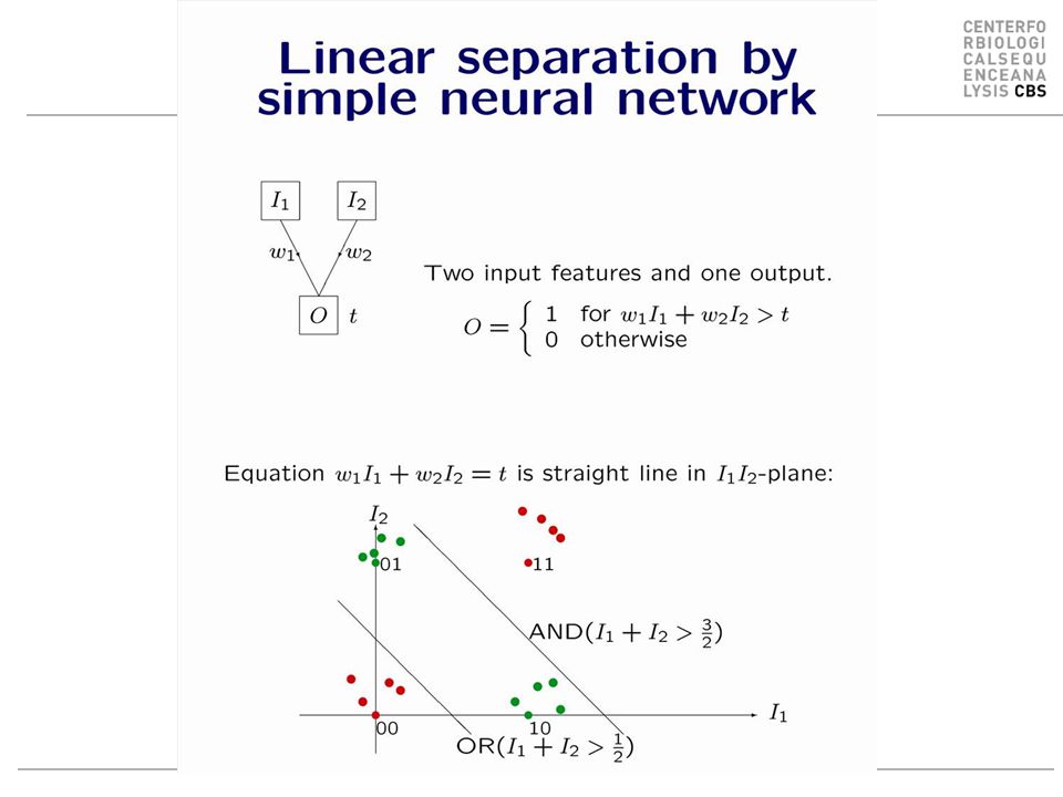
20. Neural networks Neural networks can learn higher order correlations XOR function: 0 0 => 0 1 0 => 1 0 1 => 1 1 1 => 0 (1,1) (1,0) (0,0) (0,1) No linear function can separate the points OR AND XOR

21. Error estimates XOR 0 0 => 0 1 0 => 1 0 1 => 1 1 1 => 0 (1,1) (1,0) (0,0) (0,1) Predict 0 1 Error 0 1 Mean error: 1/4

22. Neural networks v1v1 v2v2 Linear function

23. Neural networks with a hidden layer w 12 v1v1 w 21 w 22 v2v2 1 w t2 w t1 w 11 1 vtvt Input 1 (Bias) {

24. Neural network learning higher order correlations

25. Neural networks

26. How does it work? Ex. Input is (0 0) 00 6 -9 4 6 9 1 -2 -6 4 1 -4.5 Input 1 (Bias) { o 1 =-6 O 1 =0 o 2 =-2 O 2 =0 y 1 =-4.5 Y 1 =0

27. Neural networks. How does it work? Hand out

28. Neural networks (1 0 && 0 1) 10 6 -9 4 6 9 1 -2 -6 4 1 -4.5 Input 1 (Bias) { o 1 =-2 O 1 =0 o 2 =4 O 2 =1 y 1 =4.5 Y 1 =1

29. Neural networks (1 1) 11 6 -9 4 6 9 1 -2 -6 4 1 -4.5 Input 1 (Bias) { o 1 =2 O 1 =1 o 2 =10 O 2 =1 y 1 =-4.5 Y 1 =0

30. XOR function: 0 0 => 0 1 0 => 1 0 1 => 1 1 1 => 0 6 -9 4 6 9 1 -2 -6 4 1 -4.5 Input 1 (Bias) { y2y2 y1y1 What is going on?

31. (1,1) (1,0) (0,0) (0,1) x2x2 x1x1 y1y1 y2y2 (1,0) (2,2) (0,0) What is going on?

35. Network training Encoding of sequence data –Sparse encoding –Blosum encoding –Sequence profile encoding

36. Sparse encoding Inp Neuron 1 2 3 4 5 6 7 8 9 10 11 12 13 14 15 16 17 18 19 20 AAcid A 1 0 0 0 0 0 0 0 0 0 0 0 0 0 0 0 0 0 0 0 R 0 1 0 0 0 0 0 0 0 0 0 0 0 0 0 0 0 0 0 0 N 0 0 1 0 0 0 0 0 0 0 0 0 0 0 0 0 0 0 0 0 D 0 0 0 1 0 0 0 0 0 0 0 0 0 0 0 0 0 0 0 0 C 0 0 0 0 1 0 0 0 0 0 0 0 0 0 0 0 0 0 0 0 Q 0 0 0 0 0 1 0 0 0 0 0 0 0 0 0 0 0 0 0 0 E 0 0 0 0 0 0 1 0 0 0 0 0 0 0 0 0 0 0 0 0

37. BLOSUM encoding (Blosum50 matrix) A R N D C Q E G H I L K M F P S T W Y V A 4 -1 -2 -2 0 -1 -1 0 -2 -1 -1 -1 -1 -2 -1 1 0 -3 -2 0 R -1 5 0 -2 -3 1 0 -2 0 -3 -2 2 -1 -3 -2 -1 -1 -3 -2 -3 N -2 0 6 1 -3 0 0 0 1 -3 -3 0 -2 -3 -2 1 0 -4 -2 -3 D -2 -2 1 6 -3 0 2 -1 -1 -3 -4 -1 -3 -3 -1 0 -1 -4 -3 -3 C 0 -3 -3 -3 9 -3 -4 -3 -3 -1 -1 -3 -1 -2 -3 -1 -1 -2 -2 -1 Q -1 1 0 0 -3 5 2 -2 0 -3 -2 1 0 -3 -1 0 -1 -2 -1 -2 E -1 0 0 2 -4 2 5 -2 0 -3 -3 1 -2 -3 -1 0 -1 -3 -2 -2 G 0 -2 0 -1 -3 -2 -2 6 -2 -4 -4 -2 -3 -3 -2 0 -2 -2 -3 -3 H -2 0 1 -1 -3 0 0 -2 8 -3 -3 -1 -2 -1 -2 -1 -2 -2 2 -3 I -1 -3 -3 -3 -1 -3 -3 -4 -3 4 2 -3 1 0 -3 -2 -1 -3 -1 3 L -1 -2 -3 -4 -1 -2 -3 -4 -3 2 4 -2 2 0 -3 -2 -1 -2 -1 1 K -1 2 0 -1 -3 1 1 -2 -1 -3 -2 5 -1 -3 -1 0 -1 -3 -2 -2 M -1 -1 -2 -3 -1 0 -2 -3 -2 1 2 -1 5 0 -2 -1 -1 -1 -1 1 F -2 -3 -3 -3 -2 -3 -3 -3 -1 0 0 -3 0 6 -4 -2 -2 1 3 -1 P -1 -2 -2 -1 -3 -1 -1 -2 -2 -3 -3 -1 -2 -4 7 -1 -1 -4 -3 -2 S 1 -1 1 0 -1 0 0 0 -1 -2 -2 0 -1 -2 -1 4 1 -3 -2 -2 T 0 -1 0 -1 -1 -1 -1 -2 -2 -1 -1 -1 -1 -2 -1 1 5 -2 -2 0 W -3 -3 -4 -4 -2 -2 -3 -2 -2 -3 -2 -3 -1 1 -4 -3 -2 11 2 -3 Y -2 -2 -2 -3 -2 -1 -2 -3 2 -1 -1 -2 -1 3 -3 -2 -2 2 7 -1 V 0 -3 -3 -3 -1 -2 -2 -3 -3 3 1 -2 1 -1 -2 -2 0 -3 -1 4

38. Sequence encoding (continued) Sparse encoding –V:0 0 0 0 0 0 0 0 0 0 0 0 0 0 0 0 0 0 0 1 –L:0 0 0 0 0 0 0 0 1 0 0 0 0 0 0 0 0 0 0 0 –V. L=0 (unrelated) Blosum encoding –V: 0 -3 -3 -3 -1 -2 -2 -3 -3 3 1 -2 1 -1 -2 -2 0 -3 -1 4 –L:-1 -2 -3 -4 -1 -2 -3 -4 -3 2 4 -2 2 0 -3 -2 -1 -2 -1 1 –V. L = 0.88 (highly related) –V. R = -0.08 (close to unrelated)

39. Training and error reduction 

40. 

41.  Size matters

42. A Network contains a very large set of parameters –A network with 5 hidden neurons predicting binding for 9meric peptides has 9x20x5=900 weights –5 times as many weights as a matrix-based method Over fitting is a problem Use penalty for large weights (SMM) or Stop training when test performance is optimal (use early stopping) Neural network training years Temperature

43. Early stopping Maximum test set performance Most cable of generalizing

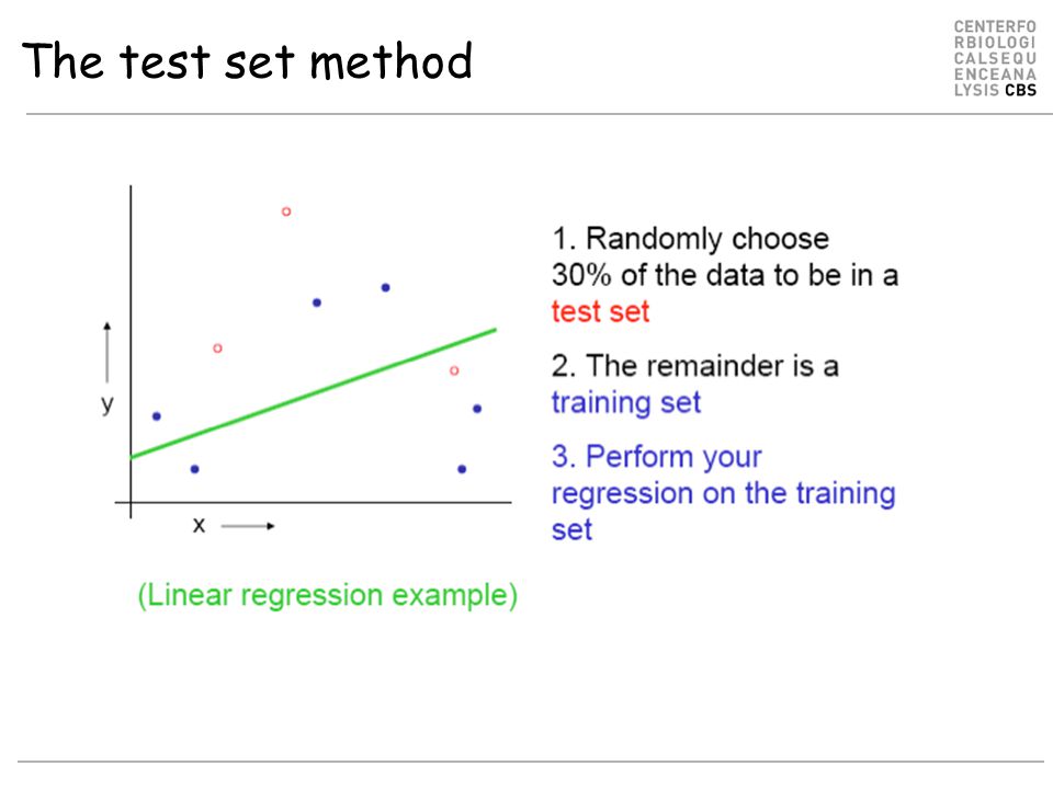
44. How to training a method. A simple statistical method: Linear regression Observations (training data): a set of x values (input) and y values (output). Model: y = ax + b (2 parameters, which are estimated from the training data)‏ Prediction: Use the model to calculate a y value for a new x value Note: the model does not fit the observations exactly. Can we do better than this?

45. Overfitting y = ax + b 2 parameter model Good description, poor fit y = ax 6 +bx 5 +cx 4 +dx 3 +ex 2 +fx+g 7 parameter model Poor description, good fit Note: It is not interesting that a model can fit its observations (training data) exactly. To function as a prediction method, a model must be able to generalize, i.e. produce sensible output on new data.

46. How to estimate parameters for prediction?

47. Model selection Linear Regression Quadratic RegressionJoin-the-dots

48. The test set method

52. So quadratic function is best

53. ALAKAAAAM ALAKAAAAN ALAKAAAAR ALAKAAAAT ALAKAAAAV GMNERPILT GILGFVFTM TLNAWVKVV KLNEPVLLL AVVPFIVSV MRSGRVHAV VRFNIDETP ANYIGQDGL AELCGDPGD QTRAVADGK GRPVPAAHP MTAQWWLDA FARGVVHVI LQRELTRLQ AVAEEMTKS Learning noise Train PSSM on raw data – No pseudo counts, No sequence weighting – Fit 9*20 parameters to 9*10 data points Evaluate on training data –PCC = 0.97 –AUC = 1.0 Close to a perfect prediction method Binders None Binders

54. AAAMAAKLA AAKNLAAAA AKALAAAAR AAAAKLATA ALAKAVAAA IPELMRTNG FIMGVFTGL NVTKVVAWL LEPLNLVLK VAVIVSVPF MRSGRVHAV VRFNIDETP ANYIGQDGL AELCGDPGD QTRAVADGK GRPVPAAHP MTAQWWLDA FARGVVHVI LQRELTRLQ AVAEEMTKS Learning noise Train PSSM on Permuted (random) data – No pseudo counts, No sequence weighting – Fit 9*20 parameters to 9*10 data points Evaluate on training data –PCC = 0.97 –AUC = 1.0 Close to a perfect prediction method AND Same performance as one the original data Binders None Binders

55. Neural network training. Cross validation Cross validation Train on 4/5 of data Test on 1/5 => Produce 5 different neural networks each with a different prediction focus

56. Early stopping Maximum test set performance Most cable of generalizing

57. The Wisdom of the Crowds The Wisdom of Crowds. Why the Many are Smarter than the Few. James Surowiecki One day in the fall of 1906, the British scientist Fracis Galton left his home and headed for a country fair… He believed that only a very few people had the characteristics necessary to keep societies healthy. He had devoted much of his career to measuring those characteristics, in fact, in order to prove that the vast majority of people did not have them. … Galton came across a weight-judging competition…Eight hundred people tried their luck. They were a diverse lot, butchers, farmers, clerks and many other no-experts…The crowd had guessed … 1.197 pounds, the ox weighted 1.198

58. Network ensembles No one single network with a particular architecture and sequence encoding scheme, will constantly perform the best Also for Neural network predictions will enlightened despotism fail –For some peptides, BLOSUM encoding with a four neuron hidden layer can best predict the peptide/MHC binding, for other peptides a sparse encoded network with zero hidden neurons performs the best –Wisdom of the Crowd Never use just one neural network Use Network ensembles

59. 5 fold training Which network to choose?

60. 5 fold training

61. Evaluation of prediction accuracy ENS : Ensemble of neural networks trained using sparse, Blosum, and weight matrix sequence encoding

62. Applications of artificial neural networks Talk recognition Prediction of protein secondary structure Prediction of Signal peptides Post translation modifications –Glycosylation –Phosphorylation Proteasomal cleavage MHC:peptide binding

64. What have we learned? Neural networks are not so bad as their reputation Neural networks can deal with higher order correlations Be careful when training a neural network –Overfitting is an important issue –Always use cross validated training