Download presentation
Presentation is loading. Please wait.

1
3 3 Chapter Numerically Summarizing Data
© 2010 Pearson Prentice Hall. All rights reserved

2
Section 3.1 Measures of Central Tendency
Objectives Determine the arithmetic mean of a variable from raw data Determine the median of a variable from raw data Explain what it means for a statistics to be resistant Determine the mode of a variable from raw data © 2010 Pearson Prentice Hall. All rights reserved 3-2

3
© 2010 Pearson Prentice Hall. All rights reserved
Objective 1 Determine the arithmetic mean of a variable from raw data © 2010 Pearson Prentice Hall. All rights reserved 3-3

4
© 2010 Pearson Prentice Hall. All rights reserved
The arithmetic mean of a variable is computed by determining the sum of all the values of the variable in the data set divided by the number of observations. © 2010 Pearson Prentice Hall. All rights reserved 3-4

5
© 2010 Pearson Prentice Hall. All rights reserved
The population arithmetic mean is computed using all the individuals in a population. The population mean is a parameter. The population arithmetic mean is denoted by . © 2010 Pearson Prentice Hall. All rights reserved 3-5

6
© 2010 Pearson Prentice Hall. All rights reserved
The sample arithmetic mean is computed using sample data. The sample mean is a statistic. The sample arithmetic mean is denoted by . © 2010 Pearson Prentice Hall. All rights reserved 3-6

7
© 2010 Pearson Prentice Hall. All rights reserved
If x1, x2, …, xN are the N observations of a variable from a population, then the population mean, µ, is © 2010 Pearson Prentice Hall. All rights reserved 3-7

8
© 2010 Pearson Prentice Hall. All rights reserved
If x1, x2, …, xn are the n observations of a variable from a sample, then the sample mean, , is © 2010 Pearson Prentice Hall. All rights reserved 3-8

9
© 2010 Pearson Prentice Hall. All rights reserved
EXAMPLE Computing a Population Mean and a Sample Mean The following data represent the travel times (in minutes) to work for all seven employees of a start-up web development company. 23, 36, 23, 18, 5, 26, 43 Compute the population mean of this data. Then take a simple random sample of n = 3 employees. Compute the sample mean. Obtain a second simple random sample of n = 3 employees. Again compute the sample mean. © 2010 Pearson Prentice Hall. All rights reserved 3-9
 to work for all seven employees of a start-up web development company. 23, 36, 23, 18, 5, 26, 43. Compute the population mean of this data. Then take a simple random sample of n = 3 employees. Compute the sample mean. Obtain a second simple random sample of n = 3 employees. Again compute the sample mean. © 2010 Pearson Prentice Hall. All rights reserved")
10
© 2010 Pearson Prentice Hall. All rights reserved
EXAMPLE Computing a Population Mean and a Sample Mean (a) © 2010 Pearson Prentice Hall. All rights reserved 3-10
 © 2010 Pearson Prentice Hall. All rights reserved")
11
© 2010 Pearson Prentice Hall. All rights reserved
EXAMPLE Computing a Population Mean and a Sample Mean (b) Obtain a simple random sample of size n = 3 from the population of seven employees. Use this simple random sample to determine a sample mean. Find a second simple random sample and determine the sample mean. 23, 36, 23, 18, 5, 26, 43 © 2010 Pearson Prentice Hall. All rights reserved 3-11
 Obtain a simple random sample of size n = 3 from the population of seven employees. Use this simple random sample to determine a sample mean. Find a second simple random sample and determine the sample mean , 36, 23, 18, 5, 26, 43. © 2010 Pearson Prentice Hall. All rights reserved")
12
© 2010 Pearson Prentice Hall. All rights reserved
3-12

13
Copyright © 2010 Pearson Education, Inc.
The lengths (in minutes) of a sample of cell phone calls are shown: Find the mean. 54 9 6 7 Copyright © 2010 Pearson Education, Inc.
 of a sample of cell phone calls are shown: Find the mean Copyright © 2010 Pearson Education, Inc.")
14
Copyright © 2010 Pearson Education, Inc.
The lengths (in minutes) of a sample of cell phone calls are shown: Find the mean. 54 9 6 7 Copyright © 2010 Pearson Education, Inc.
 of a sample of cell phone calls are shown: Find the mean Copyright © 2010 Pearson Education, Inc.")
15
© 2010 Pearson Prentice Hall. All rights reserved
Objective 2 Determine the median of a variable from raw data © 2010 Pearson Prentice Hall. All rights reserved 3-15

16
© 2010 Pearson Prentice Hall. All rights reserved
The median of a variable is the value that lies in the middle of the data when arranged in ascending order. We use M to represent the median. © 2010 Pearson Prentice Hall. All rights reserved 3-16

17
© 2010 Pearson Prentice Hall. All rights reserved
3-17

18
© 2010 Pearson Prentice Hall. All rights reserved
EXAMPLE Computing a Median of a Data Set with an Odd Number of Observations The following data represent the travel times (in minutes) to work for all seven employees of a start-up web development company. 23, 36, 23, 18, 5, 26, 43 Determine the median of this data. Step 1: 5, 18, 23, 23, 26, 36, 43 Step 2: There are n = 7 observations. M = 23 Step 3: 5, 18, 23, 23, 26, 36, 43 © 2010 Pearson Prentice Hall. All rights reserved 3-18
 to work for all seven employees of a start-up web development company. 23, 36, 23, 18, 5, 26, 43. Determine the median of this data. Step 1: 5, 18, 23, 23, 26, 36, 43. Step 2: There are n = 7 observations. M = 23. Step 3: 5, 18, 23, 23, 26, 36, 43. © 2010 Pearson Prentice Hall. All rights reserved")
19
© 2010 Pearson Prentice Hall. All rights reserved
EXAMPLE Computing a Median of a Data Set with an Even Number of Observations Suppose the start-up company hires a new employee. The travel time of the new employee is 70 minutes. Determine the median of the “new” data set. 23, 36, 23, 18, 5, 26, 43, 70 Step 1: 5, 18, 23, 23, 26, 36, 43, 70 Step 2: There are n = 8 observations. Step 3: 5, 18, 23, 23, 26, 36, 43, 70 © 2010 Pearson Prentice Hall. All rights reserved 3-19

20
Copyright © 2010 Pearson Education, Inc.
The lengths (in minutes) of a sample of cell phone calls are shown: Find the median. 3.5 9 6 7 Copyright © 2010 Pearson Education, Inc.
 of a sample of cell phone calls are shown: Find the median Copyright © 2010 Pearson Education, Inc.")
21
Copyright © 2010 Pearson Education, Inc.
The lengths (in minutes) of a sample of cell phone calls are shown: Find the median. 3.5 9 6 7 Copyright © 2010 Pearson Education, Inc.
 of a sample of cell phone calls are shown: Find the median Copyright © 2010 Pearson Education, Inc.")
22
© 2010 Pearson Prentice Hall. All rights reserved
Objective 3 Explain what it means for a statistic to be resistant © 2010 Pearson Prentice Hall. All rights reserved 3-22

23
© 2010 Pearson Prentice Hall. All rights reserved
EXAMPLE Computing a Median of a Data Set with an Even Number of Observations The following data represent the travel times (in minutes) to work for all seven employees of a start-up web development company. 23, 36, 23, 18, 5, 26, 43 Suppose a new employee is hired who has a 130 minute commute. How does this impact the value of the mean and median? Mean before new hire: 24.9 minutes Median before new hire: 23 minutes Mean after new hire: 38 minutes Median after new hire: 24.5 minutes © 2010 Pearson Prentice Hall. All rights reserved 3-23
 to work for all seven employees of a start-up web development company. 23, 36, 23, 18, 5, 26, 43. Suppose a new employee is hired who has a 130 minute commute. How does this impact the value of the mean and median Mean before new hire: 24.9 minutes Median before new hire: 23 minutes. Mean after new hire: 38 minutes Median after new hire: 24.5 minutes. © 2010 Pearson Prentice Hall. All rights reserved")
24
© 2010 Pearson Prentice Hall. All rights reserved
A numerical summary of data is said to be resistant if extreme values (very large or small) relative to the data do not affect its value substantially. © 2010 Pearson Prentice Hall. All rights reserved 3-24
 relative to the data do not affect its value substantially. © 2010 Pearson Prentice Hall. All rights reserved")
25
© 2010 Pearson Prentice Hall. All rights reserved
3-25

26
© 2010 Pearson Prentice Hall. All rights reserved
EXAMPLE Describing the Shape of the Distribution The following data represent the asking price of homes for sale in Lincoln, NE. 79,995 128,950 149,900 189,900 99,899 130,950 151,350 203,950 105,200 131,800 154,900 217,500 111,000 132,300 159,900 260,000 120,000 134,950 163,300 284,900 121,700 135,500 165,000 299,900 125,950 138,500 174,850 309,900 126,900 147,500 180,000 349,900 Source: © 2010 Pearson Prentice Hall. All rights reserved 3-26

27
© 2010 Pearson Prentice Hall. All rights reserved
Find the mean and median. Use the mean and median to identify the shape of the distribution. Verify your result by drawing a histogram of the data. © 2010 Pearson Prentice Hall. All rights reserved 3-27

28
© 2010 Pearson Prentice Hall. All rights reserved
Find the mean and median. Use the mean and median to identify the shape of the distribution. Verify your result by drawing a histogram of the data. The mean asking price is $168,320 and the median asking price is $148,700. Therefore, we would conjecture that the distribution is skewed right. © 2010 Pearson Prentice Hall. All rights reserved 3-28

29
© 2010 Pearson Prentice Hall. All rights reserved
3-29

30
© 2010 Pearson Prentice Hall. All rights reserved
Objective 4 Determine the mode of a variable from raw data © 2010 Pearson Prentice Hall. All rights reserved 3-30

31
© 2010 Pearson Prentice Hall. All rights reserved
The mode of a variable is the most frequent observation of the variable that occurs in the data set. If there is no observation that occurs with the most frequency, we say the data has no mode. © 2010 Pearson Prentice Hall. All rights reserved 3-31

32
© 2010 Pearson Prentice Hall. All rights reserved
EXAMPLE Finding the Mode of a Data Set The data on the next slide represent the Vice Presidents of the United States and their state of birth. Find the mode. © 2010 Pearson Prentice Hall. All rights reserved 3-32

33
© 2010 Pearson Prentice Hall. All rights reserved
3-33

34
© 2010 Pearson Prentice Hall. All rights reserved
3-34

35
© 2010 Pearson Prentice Hall. All rights reserved
The mode is New York. © 2010 Pearson Prentice Hall. All rights reserved 3-35

36
© 2010 Pearson Prentice Hall. All rights reserved
Tally data to determine most frequent observation © 2010 Pearson Prentice Hall. All rights reserved 3-36

37
Copyright © 2010 Pearson Education, Inc.
The lengths (in minutes) of a sample of cell phone calls are shown: Find the mode. 3 9 6 7 Copyright © 2010 Pearson Education, Inc.
 of a sample of cell phone calls are shown: Find the mode Copyright © 2010 Pearson Education, Inc.")
38
Copyright © 2010 Pearson Education, Inc.
The lengths (in minutes) of a sample of cell phone calls are shown: Find the mode. 3 9 6 7 Copyright © 2010 Pearson Education, Inc.
 of a sample of cell phone calls are shown: Find the mode Copyright © 2010 Pearson Education, Inc.")
39
Section 3.2 Measures of Dispersion
Objectives Compute the range of a variable from raw data Compute the variance of a variable from raw data Compute the standard deviation of a variable from raw data Use the Empirical Rule to describe data that are bell shaped Use Chebyshev’s Inequality to describe any data set © 2010 Pearson Prentice Hall. All rights reserved 3-39

40
© 2010 Pearson Prentice Hall. All rights reserved
To order food at a McDonald’s Restaurant, one must choose from multiple lines, while at Wendy’s Restaurant, one enters a single line. The following data represent the wait time (in minutes) in line for a simple random sample of 30 customers at each restaurant during the lunch hour. For each sample, answer the following: (a) What was the mean wait time? (b) Draw a histogram of each restaurant’s wait time. (c ) Which restaurant’s wait time appears more dispersed? Which line would you prefer to wait in? Why? © 2010 Pearson Prentice Hall. All rights reserved 3-40
 in line for a simple random sample of 30 customers at each restaurant during the lunch hour. For each sample, answer the following: (a) What was the mean wait time (b) Draw a histogram of each restaurant’s wait time. (c ) Which restaurant’s wait time appears more dispersed Which line would you prefer to wait in Why © 2010 Pearson Prentice Hall. All rights reserved")
41
© 2010 Pearson Prentice Hall. All rights reserved
Wait Time at Wendy’s Wait Time at McDonald’s © 2010 Pearson Prentice Hall. All rights reserved 3-41

42
© 2010 Pearson Prentice Hall. All rights reserved
(a) The mean wait time in each line is 1.39 minutes. © 2010 Pearson Prentice Hall. All rights reserved 3-42
 The mean wait time in each line is 1.39 minutes. © 2010 Pearson Prentice Hall. All rights reserved")
43
© 2010 Pearson Prentice Hall. All rights reserved
(b) © 2010 Pearson Prentice Hall. All rights reserved 3-43
 © 2010 Pearson Prentice Hall. All rights reserved")
44
© 2010 Pearson Prentice Hall. All rights reserved
Objective 1 Compute the range of a variable from raw data © 2010 Pearson Prentice Hall. All rights reserved 3-44

45
© 2010 Pearson Prentice Hall. All rights reserved
The range, R, of a variable is the difference between the largest data value and the smallest data values. That is Range = R = Largest Data Value – Smallest Data Value © 2010 Pearson Prentice Hall. All rights reserved 3-45

46
© 2010 Pearson Prentice Hall. All rights reserved
EXAMPLE Finding the Range of a Set of Data The following data represent the travel times (in minutes) to work for all seven employees of a start-up web development company. 23, 36, 23, 18, 5, 26, 43 Find the range. Range = 43 – 5 = 38 minutes © 2010 Pearson Prentice Hall. All rights reserved 3-46
 to work for all seven employees of a start-up web development company. 23, 36, 23, 18, 5, 26, 43. Find the range. Range = 43 – 5. = 38 minutes. © 2010 Pearson Prentice Hall. All rights reserved")
47
Copyright © 2010 Pearson Education, Inc.
The lengths (in minutes) of a sample of cell phone calls are shown: Find the range. 2 16 13 9 Copyright © 2010 Pearson Education, Inc.
 of a sample of cell phone calls are shown: Find the range Copyright © 2010 Pearson Education, Inc.")
48
Copyright © 2010 Pearson Education, Inc.
The lengths (in minutes) of a sample of cell phone calls are shown: Find the range. 2 16 13 9 Copyright © 2010 Pearson Education, Inc.
 of a sample of cell phone calls are shown: Find the range Copyright © 2010 Pearson Education, Inc.")
49
© 2010 Pearson Prentice Hall. All rights reserved
Objective 2 Compute the variance of a variable from raw data © 2010 Pearson Prentice Hall. All rights reserved 3-49

50
© 2010 Pearson Prentice Hall. All rights reserved
The population variance of a variable is the sum of squared deviations about the population mean divided by the number of observations in the population, N. That is it is the mean of the sum of the squared deviations about the population mean. © 2010 Pearson Prentice Hall. All rights reserved 3-50

51
© 2010 Pearson Prentice Hall. All rights reserved
The population variance is symbolically represented by σ2 (lower case Greek sigma squared). Note: When using the above formula, do not round until the last computation. Use as many decimals as allowed by your calculator in order to avoid round off errors. © 2010 Pearson Prentice Hall. All rights reserved 3-51
. Note: When using the above formula, do not round until the last computation. Use as many decimals as allowed by your calculator in order to avoid round off errors. © 2010 Pearson Prentice Hall. All rights reserved")
52
© 2010 Pearson Prentice Hall. All rights reserved
EXAMPLE Computing a Population Variance The following data represent the travel times (in minutes) to work for all seven employees of a start-up web development company. 23, 36, 23, 18, 5, 26, 43 Compute the population variance of this data. Recall that © 2010 Pearson Prentice Hall. All rights reserved 3-52
 to work for all seven employees of a start-up web development company. 23, 36, 23, 18, 5, 26, 43. Compute the population variance of this data. Recall that. © 2010 Pearson Prentice Hall. All rights reserved")
53
© 2010 Pearson Prentice Hall. All rights reserved
xi μ xi – μ (xi – μ)2 23 36 18 5 26 43 minutes2 © 2010 Pearson Prentice Hall. All rights reserved 3-53
 minutes2. © 2010 Pearson Prentice Hall. All rights reserved")
54
The Computational Formula
© 2010 Pearson Prentice Hall. All rights reserved 3-54

55
© 2010 Pearson Prentice Hall. All rights reserved
EXAMPLE Computing a Population Variance Using the Computational Formula The following data represent the travel times (in minutes) to work for all seven employees of a start-up web development company. 23, 36, 23, 18, 5, 26, 43 Compute the population variance of this data using the computational formula. © 2010 Pearson Prentice Hall. All rights reserved 3-55
 to work for all seven employees of a start-up web development company. 23, 36, 23, 18, 5, 26, 43. Compute the population variance of this data using the computational formula. © 2010 Pearson Prentice Hall. All rights reserved")
56
© 2010 Pearson Prentice Hall. All rights reserved
23, 36, 23, 18, 5, 26, 43 © 2010 Pearson Prentice Hall. All rights reserved 3-56

57
© 2010 Pearson Prentice Hall. All rights reserved
The sample variance is computed by determining the sum of squared deviations about the sample mean and then dividing this result by n – 1. © 2010 Pearson Prentice Hall. All rights reserved 3-57

58
© 2010 Pearson Prentice Hall. All rights reserved
Note: Whenever a statistic consistently overestimates or underestimates a parameter, it is called biased. To obtain an unbiased estimate of the population variance, we divide the sum of the squared deviations about the mean by n - 1. © 2010 Pearson Prentice Hall. All rights reserved 3-58

59
EXAMPLE Computing a Sample Variance
In Section 3.1, we obtained the following simple random sample for the travel time data: 5, 36, 26. Compute the sample variance travel time. Travel Time, xi Sample Mean, Deviation about the Mean, Squared Deviations about the Mean, 5 22.333 5 – = ( )2 = 36 13.667 26 3.667 square minutes © 2010 Pearson Prentice Hall. All rights reserved 3-59
2 = square minutes. © 2010 Pearson Prentice Hall. All rights reserved")
60
© 2010 Pearson Prentice Hall. All rights reserved
Objective 3 Compute the standard deviation of a variable from raw data © 2010 Pearson Prentice Hall. All rights reserved 3-60

61
© 2010 Pearson Prentice Hall. All rights reserved
The population standard deviation is denoted by It is obtained by taking the square root of the population variance, so that The sample standard deviation is denoted by s It is obtained by taking the square root of the sample variance, so that © 2010 Pearson Prentice Hall. All rights reserved 3-61

62
© 2010 Pearson Prentice Hall. All rights reserved
EXAMPLE Computing a Population Standard Deviation The following data represent the travel times (in minutes) to work for all seven employees of a start-up web development company. 23, 36, 23, 18, 5, 26, 43 Compute the population standard deviation of this data. Recall, from the last objective that σ2 = minutes2. Therefore, © 2010 Pearson Prentice Hall. All rights reserved 3-62
 to work for all seven employees of a start-up web development company. 23, 36, 23, 18, 5, 26, 43. Compute the population standard deviation of this data. Recall, from the last objective that σ2 = minutes2. Therefore, © 2010 Pearson Prentice Hall. All rights reserved")
63
© 2010 Pearson Prentice Hall. All rights reserved
EXAMPLE Computing a Sample Standard Deviation Recall the sample data 5, 26, 36 results in a sample variance of square minutes Use this result to determine the sample standard deviation. © 2010 Pearson Prentice Hall. All rights reserved 3-63

64
Copyright © 2010 Pearson Education, Inc.
The lengths (in minutes) of a sample of cell phone calls are shown: Find the standard deviation. 5.7 5.2 32.8 16 Copyright © 2010 Pearson Education, Inc.
 of a sample of cell phone calls are shown: Find the standard deviation Copyright © 2010 Pearson Education, Inc.")
65
Copyright © 2010 Pearson Education, Inc.
The lengths (in minutes) of a sample of cell phone calls are shown: Find the standard deviation. 5.7 5.2 32.8 16 Copyright © 2010 Pearson Education, Inc.
 of a sample of cell phone calls are shown: Find the standard deviation Copyright © 2010 Pearson Education, Inc.")
66
© 2010 Pearson Prentice Hall. All rights reserved
EXAMPLE Comparing Standard Deviations Determine the standard deviation waiting time for Wendy’s and McDonald’s. Which is larger? Why? © 2010 Pearson Prentice Hall. All rights reserved 3-66

67
© 2010 Pearson Prentice Hall. All rights reserved
Wait Time at Wendy’s Wait Time at McDonald’s © 2010 Pearson Prentice Hall. All rights reserved 3-67

68
© 2010 Pearson Prentice Hall. All rights reserved
EXAMPLE Comparing Standard Deviations Determine the standard deviation waiting time for Wendy’s and McDonald’s. Which is larger? Why? Sample standard deviation for Wendy’s: 0.738 minutes Sample standard deviation for McDonald’s: 1.265 minutes © 2010 Pearson Prentice Hall. All rights reserved 3-68

69
© 2010 Pearson Prentice Hall. All rights reserved
Objective 4 Use the Empirical Rule to Describe Data That Are Bell Shaped © 2010 Pearson Prentice Hall. All rights reserved 3-69

70
© 2010 Pearson Prentice Hall. All rights reserved
3-70

71
© 2010 Pearson Prentice Hall. All rights reserved
3-71

72
© 2010 Pearson Prentice Hall. All rights reserved
EXAMPLE Using the Empirical Rule The following data represent the serum HDL cholesterol of the 54 female patients of a family doctor. © 2010 Pearson Prentice Hall. All rights reserved 3-72

73
© 2010 Pearson Prentice Hall. All rights reserved
(a) Compute the population mean and standard deviation. (b) Draw a histogram to verify the data is bell-shaped. (c) Determine the percentage of patients that have serum HDL within 3 standard deviations of the mean according to the Empirical Rule. (d) Determine the percentage of patients that have serum HDL between 34 and 69.1 according to the Empirical Rule. (e) Determine the actual percentage of patients that have serum HDL between 34 and 69.1. © 2010 Pearson Prentice Hall. All rights reserved 3-73
 Compute the population mean and standard deviation. (b) Draw a histogram to verify the data is bell-shaped. (c) Determine the percentage of patients that have serum HDL within 3 standard deviations of the mean according to the Empirical Rule. (d) Determine the percentage of patients that have serum HDL between 34 and 69.1 according to the Empirical Rule. (e) Determine the actual percentage of patients that have serum HDL between 34 and © 2010 Pearson Prentice Hall. All rights reserved")
74
© 2010 Pearson Prentice Hall. All rights reserved
(a) Using a TI-83 plus graphing calculator, we find (b) © 2010 Pearson Prentice Hall. All rights reserved 3-74
 Using a TI-83 plus graphing calculator, we find. (b) © 2010 Pearson Prentice Hall. All rights reserved")
75
© 2010 Pearson Prentice Hall. All rights reserved
(c) According to the Empirical Rule, 99.7% of the patients that have serum HDL within 3 standard deviations of the mean. (d) 13.5% + 34% + 34% = 81.5% of patients will have a serum HDL between 34.0 and 69.1 according to the Empirical Rule. (e) 45 out of the 54 or 83.3% of the patients have a serum HDL between 34.0 and 69.1. © 2010 Pearson Prentice Hall. All rights reserved 3-75
 According to the Empirical Rule, 99.7% of the patients that have serum HDL within 3 standard deviations of the mean. (d) 13.5% + 34% + 34% = 81.5% of patients will have a serum HDL between 34.0 and 69.1 according to the Empirical Rule. (e) 45 out of the 54 or 83.3% of the patients have a serum HDL between 34.0 and © 2010 Pearson Prentice Hall. All rights reserved")
76
Copyright © 2010 Pearson Education, Inc.
The mean commute time in the U.S. is 24.4 minutes with a standard deviation of 6.5 minutes. What is the minimum percentage of commuters that have commute times between 11.4 minutes and 37.4 minutes? 68% 75% 89% 95% Copyright © 2010 Pearson Education, Inc.

77
Copyright © 2010 Pearson Education, Inc.
The mean commute time in the U.S. is 24.4 minutes with a standard deviation of 6.5 minutes. What is the minimum percentage of commuters that have commute times between 11.4 minutes and 37.4 minutes? 68% 75% 89% 95% Copyright © 2010 Pearson Education, Inc.

78
© 2010 Pearson Prentice Hall. All rights reserved
Objective 5 Use Chebyshev’s Inequality to Describe Any Set of Data © 2010 Pearson Prentice Hall. All rights reserved 3-78

79
© 2010 Pearson Prentice Hall. All rights reserved
3-79

80
© 2010 Pearson Prentice Hall. All rights reserved
EXAMPLE Using Chebyshev’s Theorem Using the data from the previous example, use Chebyshev’s Theorem to determine the percentage of patients that have serum HDL within 3 standard deviations of the mean. (b) determine the actual percentage of patients that have serum HDL between 34 and 80.8. © 2010 Pearson Prentice Hall. All rights reserved 3-80
 determine the actual percentage of patients that have serum HDL between 34 and © 2010 Pearson Prentice Hall. All rights reserved")
81
© 2010 Pearson Prentice Hall. All rights reserved
Section Measures of Central Tendency and Dispersion from Grouped Data Objectives Approximate the mean of a variable from grouped data Compute the weighted mean Approximate the variance and standard deviation of a variable from grouped data © 2010 Pearson Prentice Hall. All rights reserved 3-81

82
© 2010 Pearson Prentice Hall. All rights reserved
Objective 1 Approximate the Mean of a Variable from Grouped Data © 2010 Pearson Prentice Hall. All rights reserved 3-82

83
© 2010 Pearson Prentice Hall. All rights reserved
3-83

84
© 2010 Pearson Prentice Hall. All rights reserved
EXAMPLE Approximating the Mean from a Relative Frequency Distribution The National Survey of Student Engagement is a survey that (among other things) asked first year students at liberal arts colleges how much time they spend preparing for class each week. The results from the 2007 survey are summarized below. Approximate the mean number of hours spent preparing for class each week. Hours 1-5 6-10 11-15 16-20 21-25 26-30 31-35 Frequency 130 250 230 180 100 60 50 Source: © 2010 Pearson Prentice Hall. All rights reserved 3-84
 asked first year students at liberal arts colleges how much time they spend preparing for class each week. The results from the 2007 survey are summarized below. Approximate the mean number of hours spent preparing for class each week. Hours Frequency Source: © 2010 Pearson Prentice Hall. All rights reserved")
85
© 2010 Pearson Prentice Hall. All rights reserved
Time Frequency xi xi fi 1 - 5 130 3.5 455 6 - 10 250 8.5 2125 230 13.5 3105 180 18.5 3330 100 23.5 2350 26 – 30 60 28.5 1710 31 – 35 50 33.5 1675 © 2010 Pearson Prentice Hall. All rights reserved 3-85

86
Copyright © 2010 Pearson Education, Inc.
Approximate the mean of the frequency distribution. 13 19.5 9.5 12.5 Class Frequency, f 1 – 6.99 21 7 – 12.99 16 13 – 18.99 28 19 – 24.99 13 Copyright © 2010 Pearson Education, Inc.

87
Copyright © 2010 Pearson Education, Inc.
Approximate the mean of the frequency distribution. 13 19.5 9.5 12.5 Class Frequency, f 1 – 6.99 21 7 – 12.99 16 13 – 18.99 28 19 – 24.99 13 Copyright © 2010 Pearson Education, Inc.

88
© 2010 Pearson Prentice Hall. All rights reserved
Objective 2 Compute the Weighted Mean © 2010 Pearson Prentice Hall. All rights reserved 3-88

89
© 2010 Pearson Prentice Hall. All rights reserved
3-89

90
© 2010 Pearson Prentice Hall. All rights reserved
EXAMPLE Computed a Weighted Mean Bob goes the “Buy the Weigh” Nut store and creates his own bridge mix. He combines 1 pound of raisins, 2 pounds of chocolate covered peanuts, and 1.5 pounds of cashews. The raisins cost $1.25 per pound, the chocolate covered peanuts cost $3.25 per pound, and the cashews cost $5.40 per pound. What is the cost per pound of this mix. © 2010 Pearson Prentice Hall. All rights reserved 3-90

91
© 2010 Pearson Prentice Hall. All rights reserved
Objective 3 Approximate the Variance and Standard Deviation of a Variable from Grouped Data © 2010 Pearson Prentice Hall. All rights reserved 3-91

92
© 2010 Pearson Prentice Hall. All rights reserved
3-92

93
© 2010 Pearson Prentice Hall. All rights reserved
EXAMPLE Approximating the Mean from a Relative Frequency Distribution The National Survey of Student Engagement is a survey that (among other things) asked first year students at liberal arts colleges how much time they spend preparing for class each week. The results from the 2007 survey are summarized below. Approximate the variance and standard deviation number of hours spent preparing for class each week. Hours 1-5 6-10 11-15 16-20 21-25 26-30 31-35 Frequency 130 250 230 180 100 60 50 Source: © 2010 Pearson Prentice Hall. All rights reserved 3-93
 asked first year students at liberal arts colleges how much time they spend preparing for class each week. The results from the 2007 survey are summarized below. Approximate the variance and standard deviation number of hours spent preparing for class each week. Hours Frequency Source: © 2010 Pearson Prentice Hall. All rights reserved")
94
© 2010 Pearson Prentice Hall. All rights reserved
Time Frequency x 3.5 1 - 5 130 6 - 10 250 8.5 230 13.5 180 18.5 100 23.5 60 28.5 50 33.5 © 2010 Pearson Prentice Hall. All rights reserved 3-94

95
Objectives Section 3.4 Measures of Position and Outliers
Determine and interpret z-scores Interpret percentiles Determine and interpret quartiles Determine and interpret the interquartile range Check a set of data for outliers © 2010 Pearson Prentice Hall. All rights reserved 3-95

96
© 2010 Pearson Prentice Hall. All rights reserved
3-96

97
EXAMPLE Using Z-Scores
The mean height of males 20 years or older is 69.1 inches with a standard deviation of 2.8 inches. The mean height of females 20 years or older is 63.7 inches with a standard deviation of 2.7 inches. Data based on information obtained from National Health and Examination Survey. Who is relatively taller? Kevin Garnett whose height is 83 inches or Candace Parker whose height is 76 inches © 2010 Pearson Prentice Hall. All rights reserved 3-97

98
© 2010 Pearson Prentice Hall. All rights reserved
Kevin Garnett’s height is 4.96 standard deviations above the mean. Candace Parker’s height is 4.56 standard deviations above the mean. Kevin Garnett is relatively taller. © 2010 Pearson Prentice Hall. All rights reserved 3-98

99
Copyright © 2010 Pearson Education, Inc.
The mean commute time in the U.S. is 24.4 minutes with a standard deviation of 6.5 minutes. Find the z-score that corresponds to a commute time of 15 minutes. 1.45 –1.45 11.25 –9.4 Copyright © 2010 Pearson Education, Inc.

100
Copyright © 2010 Pearson Education, Inc.
The mean commute time in the U.S. is 24.4 minutes with a standard deviation of 6.5 minutes. Find the z-score that corresponds to a commute time of 15 minutes. 1.45 –1.45 11.25 –9.4 Copyright © 2010 Pearson Education, Inc.

101
Copyright © 2010 Pearson Education, Inc.
The mean commute time in the U.S. is 24.4 minutes with a standard deviation of 6.5 minutes. Find the z-score that corresponds to a commute time of 15 minutes. 1.45 –1.45 11.25 –9.4 Copyright © 2010 Pearson Education, Inc.

102
Copyright © 2010 Pearson Education, Inc.
The mean commute time in the U.S. is 24.4 minutes with a standard deviation of 6.5 minutes. Find the z-score that corresponds to a commute time of 15 minutes. 1.45 –1.45 11.25 –9.4 Copyright © 2010 Pearson Education, Inc.

103
© 2010 Pearson Prentice Hall. All rights reserved
Objective 2 Interpret Percentiles © 2010 Pearson Prentice Hall. All rights reserved 3-103

104
© 2010 Pearson Prentice Hall. All rights reserved
The kth percentile, denoted, Pk, of a set of data is a value such that k percent of the observations are less than or equal to the value. © 2010 Pearson Prentice Hall. All rights reserved 3-104

105
© 2010 Pearson Prentice Hall. All rights reserved
EXAMPLE Interpret a Percentile The Graduate Record Examination (GRE) is a test required for admission to many U.S. graduate schools. The University of Pittsburgh Graduate School of Public Health requires a GRE score no less than the 70th percentile for admission into their Human Genetics MPH or MS program. (Source: Interpret this admissions requirement. In general, the 70th percentile is the score such that 70% of the individuals who took the exam scored worse, and 30% of the individuals scores better. In order to be admitted to this program, an applicant must score as high or higher than 70% of the people who take the GRE. Put another way, the individual’s score must be in the top 30%. © 2010 Pearson Prentice Hall. All rights reserved 3-105
 is a test required for admission to many U.S. graduate schools. The University of Pittsburgh Graduate School of Public Health requires a GRE score no less than the 70th percentile for admission into their Human Genetics MPH or MS program. (Source: pageID=101.) Interpret this admissions requirement. In general, the 70th percentile is the score such that 70% of the individuals who took the exam scored worse, and 30% of the individuals scores better. In order to be admitted to this program, an applicant must score as high or higher than 70% of the people who take the GRE. Put another way, the individual’s score must be in the top 30%. © 2010 Pearson Prentice Hall. All rights reserved")
106
© 2010 Pearson Prentice Hall. All rights reserved
Objective 3 Determine and Interpret Quartiles © 2010 Pearson Prentice Hall. All rights reserved 3-106

107
© 2010 Pearson Prentice Hall. All rights reserved
Quartiles divide data sets into fourths, or four equal parts. The 1st quartile, denoted Q1, divides the bottom 25% the data from the top 75%. Therefore, the 1st quartile is equivalent to the 25th percentile. The 2nd quartile divides the bottom 50% of the data from the top 50% of the data, so that the 2nd quartile is equivalent to the 50th percentile, which is equivalent to the median. The 3rd quartile divides the bottom 75% of the data from the top 25% of the data, so that the 3rd quartile is equivalent to the 75th percentile. © 2010 Pearson Prentice Hall. All rights reserved 3-107

108
© 2010 Pearson Prentice Hall. All rights reserved
3-108

109
© 2010 Pearson Prentice Hall. All rights reserved
EXAMPLE Finding and Interpreting Quartiles A group of Brigham Young University—Idaho students (Matthew Herring, Nathan Spencer, Mark Walker, and Mark Steiner) collected data on the speed of vehicles traveling through a construction zone on a state highway, where the posted speed was 25 mph. The recorded speed of 14 randomly selected vehicles is given below: 20, 24, 27, 28, 29, 30, 32, 33, 34, 36, 38, 39, 40, 40 Find and interpret the quartiles for speed in the construction zone. Step 1: The data is already in ascending order. Step 2: There are n = 14 observations, so the median, or second quartile, Q2, is the mean of the 7th and 8th observations. Therefore, M = 32.5. Step 3: The median of the bottom half of the data is the first quartile, Q1. 20, 24, 27, 28, 29, 30, 32 The median of these seven observations is 28. Therefore, Q1 = 28. The median of the top half of the data is the third quartile, Q3. Therefore, Q3 = 38. © 2010 Pearson Prentice Hall. All rights reserved 3-109
 collected data on the speed of vehicles traveling through a construction zone on a state highway, where the posted speed was 25 mph. The recorded speed of 14 randomly selected vehicles is given below: 20, 24, 27, 28, 29, 30, 32, 33, 34, 36, 38, 39, 40, 40. Find and interpret the quartiles for speed in the construction zone. Step 1: The data is already in ascending order. Step 2: There are n = 14 observations, so the median, or second quartile, Q2, is the mean of the 7th and 8th observations. Therefore, M = Step 3: The median of the bottom half of the data is the first quartile, Q1. 20, 24, 27, 28, 29, 30, 32. The median of these seven observations is 28. Therefore, Q1 = 28. The median of the top half of the data is the third quartile, Q3. Therefore, Q3 = 38. © 2010 Pearson Prentice Hall. All rights reserved")
110
© 2010 Pearson Prentice Hall. All rights reserved
Interpretation: 25% of the speeds are less than or equal to the first quartile, 28 miles per hour, and 75% of the speeds are greater than 28 miles per hour. 50% of the speeds are less than or equal to the second quartile, 32.5 miles per hour, and 50% of the speeds are greater than 32.5 miles per hour. 75% of the speeds are less than or equal to the third quartile, 38 miles per hour, and 25% of the speeds are greater than 38 miles per hour. © 2010 Pearson Prentice Hall. All rights reserved 3-110

111
© 2010 Pearson Prentice Hall. All rights reserved
Objective 4 Determine and Interpret the Interquartile Range © 2010 Pearson Prentice Hall. All rights reserved 3-111

112
© 2010 Pearson Prentice Hall. All rights reserved
3-112

113
© 2010 Pearson Prentice Hall. All rights reserved
EXAMPLE Determining and Interpreting the Interquartile Range Determine and interpret the interquartile range of the speed data. Q1 = Q3 = 38 The range of the middle 50% of the speed of cars traveling through the construction zone is 10 miles per hour. © 2010 Pearson Prentice Hall. All rights reserved 3-113

114
© 2010 Pearson Prentice Hall. All rights reserved
Suppose a 15th car travels through the construction zone at 100 miles per hour. How does this value impact the mean, median, standard deviation, and interquartile range? Without 15th car With 15th car Mean 32.1 mph 36.7 mph Median 32.5 mph 33 mph Standard deviation 6.2 mph 18.5 mph IQR 10 mph 11 mph © 2010 Pearson Prentice Hall. All rights reserved 3-114

115
Copyright © 2010 Pearson Education, Inc.
The closing prices for 9 telecommunications stocks are shown below. Compute the interquartile range, IQR. 29.845 68.32 6.21 36.055 Copyright © 2010 Pearson Education, Inc.

116
Copyright © 2010 Pearson Education, Inc.
The closing prices for 9 telecommunications stocks are shown below. Compute the interquartile range, IQR. 29.845 68.32 6.21 36.055 Copyright © 2010 Pearson Education, Inc.

117
© 2010 Pearson Prentice Hall. All rights reserved
Objective 5 Check a Set of Data for Outliers © 2010 Pearson Prentice Hall. All rights reserved 3-117

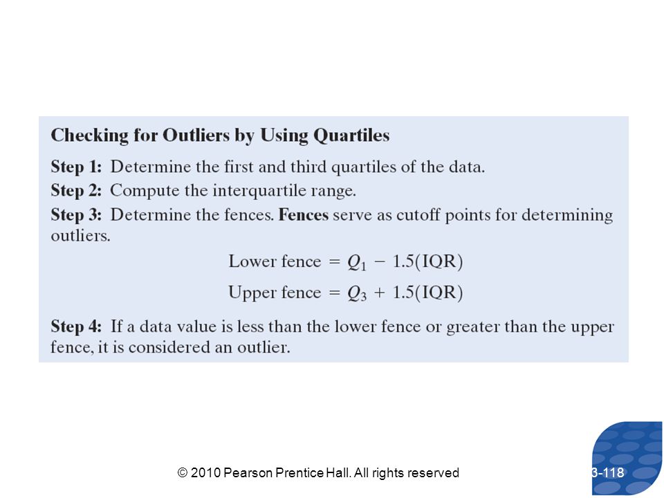
118
© 2010 Pearson Prentice Hall. All rights reserved
3-118
119
© 2010 Pearson Prentice Hall. All rights reserved
EXAMPLE Determining and Interpreting the Interquartile Range Check the speed data for outliers. Step 1: The first and third quartiles are Q1 = 28 mph and Q3 = 38 mph. Step 2: The interquartile range is 10 mph. Step 3: The fences are Lower Fence = Q1 – 1.5(IQR) Upper Fence = Q (IQR) = 28 – 1.5(10) = (10) = 13 mph = 53 mph Step 4: There are no values less than 13 mph or greater than 53 mph. Therefore, there are no outliers. © 2010 Pearson Prentice Hall. All rights reserved 3-119
 Upper Fence = Q (IQR) = 28 – 1.5(10) = (10) = 13 mph = 53 mph. Step 4: There are no values less than 13 mph or greater than 53 mph. Therefore, there are no outliers. © 2010 Pearson Prentice Hall. All rights reserved")
120
Objectives Compute the five-number summary Draw and interpret boxplots
Section 3.5 The Five-Number Summary and Boxplots Objectives Compute the five-number summary Draw and interpret boxplots © 2010 Pearson Prentice Hall. All rights reserved 3-120

121
© 2010 Pearson Prentice Hall. All rights reserved
3-121

122
© 2010 Pearson Prentice Hall. All rights reserved
EXAMPLE Obtaining the Five-Number Summary Every six months, the United States Federal Reserve Board conducts a survey of credit card plans in the U.S. The following data are the interest rates charged by 10 credit card issuers randomly selected for the July 2005 survey. Determine the five-number summary of the data. First, we write the data is ascending order: 6.5%, 9.9%, 12.0%, 13.0%, 13.3%, 13.9%, 14.3%, 14.4%, 14.4%, 14.5% Institution Rate Pulaski Bank and Trust Company 6.5% Rainier Pacific Savings Bank 12.0% Wells Fargo Bank NA 14.4% Firstbank of Colorado Lafayette Ambassador Bank 14.3% Infibank 13.0% United Bank, Inc. 13.3% First National Bank of The Mid-Cities 13.9% Bank of Louisiana 9.9% Bar Harbor Bank and Trust Company 14.5% The smallest number is 6.5%. The largest number is 14.5%. The first quartile is 12.0%. The second quartile is 13.6%. The third quartile is 14.4%. Five-number Summary: 6.5% 12.0% 13.6% 14.4% 14.5% Source: © 2010 Pearson Prentice Hall. All rights reserved 3-122

123
© 2010 Pearson Prentice Hall. All rights reserved
Objective 2 Draw and interpret boxplots © 2010 Pearson Prentice Hall. All rights reserved 3-123

124
© 2010 Pearson Prentice Hall. All rights reserved
3-124

125
© 2010 Pearson Prentice Hall. All rights reserved
EXAMPLE Constructing a Boxplot Every six months, the United States Federal Reserve Board conducts a survey of credit card plans in the U.S. The following data are the interest rates charged by 10 credit card issuers randomly selected for the July 2005 survey. Draw a boxplot of the data. Institution Rate Pulaski Bank and Trust Company 6.5% Rainier Pacific Savings Bank 12.0% Wells Fargo Bank NA 14.4% Firstbank of Colorado Lafayette Ambassador Bank 14.3% Infibank 13.0% United Bank, Inc. 13.3% First National Bank of The Mid-Cities 13.9% Bank of Louisiana 9.9% Bar Harbor Bank and Trust Company 14.5% Source: © 2010 Pearson Prentice Hall. All rights reserved 3-125

126
Step 1: The interquartile range (IQR) is 14. 4% - 12% = 2. 4%
Step 1: The interquartile range (IQR) is 14.4% - 12% = 2.4%. The lower and upper fences are: Lower Fence = Q1 – 1.5(IQR) Upper Fence = Q (IQR) = 12 – 1.5(2.4) = (2.4) = 8.4% = 18.0% Step 2: * [ ] © 2010 Pearson Prentice Hall. All rights reserved 3-126
 is 14.4% - 12% = 2.4%. The lower and upper fences are: Lower Fence = Q1 – 1.5(IQR) Upper Fence = Q (IQR) = 12 – 1.5(2.4) = (2.4) = 8.4% = 18.0% Step 2: * [ ] © 2010 Pearson Prentice Hall. All rights reserved")
127
© 2010 Pearson Prentice Hall. All rights reserved
Objective 3 Use a boxplot and quartiles to describe the shape of a distribution © 2010 Pearson Prentice Hall. All rights reserved 3-127

128
© 2010 Pearson Prentice Hall. All rights reserved
The interest rate boxplot indicates that the distribution is skewed left. © 2010 Pearson Prentice Hall. All rights reserved 3-128

129
Copyright © 2010 Pearson Education, Inc.
Use the boxplot to identify the first quartile. 10 18 24 26 10 18 24 26 30 | | | | | | | | | | | Copyright © 2010 Pearson Education, Inc.

130
Copyright © 2010 Pearson Education, Inc.
Use the boxplot to identify the first quartile. 10 18 24 26 10 18 24 26 30 | | | | | | | | | | | Copyright © 2010 Pearson Education, Inc.

Similar presentations


 Grants Chapter 6.>")


 Geometry (29%)>")

