1. Meta-analysis in animal health and reproduction: methods and applications using Stata
Ahmad Rabiee
Ian Lean
PO Box 660
Camden 2570, NSW
SBScibus.com.au

3. Meta-analysis Literature search study quality assessment
Selection criteria
Statistical analysis
Heterogeneity
Publication bias

4. Methods of pooling study results
Narrative procedure (conventional critical review method)
Vote-counting method (significant results marked “+”, converse “–” and no significant results “neutral”)
Combined tests (combining the probabilities obtain from two or more independent studies)

5. Systematic Reviews & Meta-analysis
Systematic review is the entire process of collecting, reviewing and presenting all available evidence
Meta-analysis is the statistical technique involved in extracting and combining data to produce a summary result

6. Meta-analysis
A meta-analysis is also possible without doing a systematic review
With no attempt to be systematic about the particular studies were chosen

7. Aim of a meta-analysis To increase power To improve precision
To answer questions not posed by the individual studies
To settle controversies arising from apparently conflicting studies or
To generate new hypothesis

8. Objective of a meta-analysis
Assessment of strength of evidence
To determine whether an effect exists in a particular direction
Statistical pooling of results
To obtain a single summary result
Investigation of heterogeneity
To examine reasons for different results

9. Meta-analysis A meta-analysis is a two-stage process Stage 1 Stage 2
Extraction of data from individual study
Calculation of a result for that study (point estimate)
Estimation of chance variation (confidence interval)
Stage 2
Deciding if it is appropriate to calculate and pool average results across studies
If so, calculate and present the results.

10. Analysis specification
What are the main comparisons in your view?
How will you summarise the results of the outcomes for each study?
How will you decide whether to combine the results of the separate studies?
Do you plan any subgroup or sensitivity analyses?

11. Different types of data
Dichotomous data (e.g. dead or live)
Counts of events (e.g. no. of pregnancies)
Short ordinal scales (e.g. pain score)
Long ordinal scales (e.g. quality of life)
Continuous data (e.g. cholesterol con.)
Censored data or survival data (e.g. time to 1st service)

12. Methods of calculating summary measures of association or effect
Continuous data
Calculation of overall effect size (standardised mean difference)
Rate data
Measures of effect (difference between incidence in the population of exposed vs not exposed)
Relative risk
Odds ratio
Risk difference

13. Statistical models Fixed effect models Random effect models
Mantel-Haenszel (MH)
Has optimal statistical power
Softwares are available for the analysis
Peto test (modified MH method)
Recommended for non-experimental studies
Random effect models
DerSimonian & Laird method
Bayesian method
Regression models (Mixed model)

14. Fixed effect model
This model is based on a mathematical assumption that every study is evaluating a common treatment effect
In this model, the true treatment difference is considered to be the same for all trials
The SE of each trial estimate is based on sampling variation within the trial
The summary results are specific to the trials included
The summary results can not be generalised to the population

15. Fixed effect methods Mantel-Haenszel approach Odd ratio Risk ratio
Risk difference
Not recommended in review with sparse data (trials with zero events in treatment or control group)
Peto method
Odds ratio
Used in studies with small treatment effect and rare events
Not a very common method
Used when the size of groups within trial are balanced
If the results from the trials appear to be reasonably consistent the fixed effects analysis may be more appropriate one to present.
For a MA based on a small number of studies, the estimate of the heterogeneity parameters from the data is likely to be unreliable.

16. Random effect model
In this model, the assumption is that the true treatment effects in the individual studies may be different from each other
In this model, the true treatment difference in each trial is itself assumed to be a realisation of random variable, which is usually assumed to be normally distributed
The SE of each trial estimate is increased due to the addition of this between-trial variation
For a MA based on a larger number of trials the random effect analysis may be preferred anyway.
There are some concerns regarding the use of the random effect model in practice;
1- First, the random effects model assumes that the results from the trials included in the MA are representative of the results would be obtained from the total population of treatment centres. In reality, centres which take part in clinical trials are not chosen at random.
2- Second, when there are only a few trials for inclusion in the meta-analysis, it may inappropriate to try to fit a random effects model as any calculated estimate of the between study variance will be unreliable. When there is only one available trial, its analysis can only be based on fixed effects model.

17. Random effects analytic methods
Odd ratio
Risk ratio
Risk difference

18. Fixed effect vs Random effect
Fixed effects assumption
“did the treatment produce benefit on average in the studies in hand”?
“what is the best estimate of the treatment effect”?
Random effects assumption
“will the treatment produce benefit on average”?
“what is the average treatment effect”?
Choice between fixed and random effects may be decided
By a formal chi-square test of homogeneity
That is whether the between study variance component is zero or not

19. Dichotomous data Risk Odds
A chance or probability of having a specific event (no of participants having the event in a group divided the total no. of participants)
Odds
The ratio of events to not-events (risk of having an events divided by the risk of not having it)

20. Dichotomous data Odds Ratio (OR) Relative risk or Risk Ratio (RR)
The odds of the event occurring in one group divided by the odds of the event occurring in the other group
Relative risk or Risk Ratio (RR)
The risk of the events in one group divided by the risk of the event in the other group
Risk difference (RD; -1 to +1)
Risk in the experimental group minus risk in the control group
Confidence interval (CI)
The level of uncertainty in the estimate of treatment effect
An estimate of the range in which the estimate would fall a fixed percentage of times if the study repeated many times
RR: The risk of still being infected on antibiotic was about 12% of the risk on control OR
RR: Treatment reduced the risk to 12% of what it would have been
_______________________________________________
OR: Antibiotics reduced the odds of still being infected to about 2% of what they would have been
OR: Treatment reduced the odds by 88% of what they were in the control group.
_________________________________________________
RD: Antibiotics reduced the risk of still being infected by 76% points.
Switching between good and bad outcomes for the risk difference causes a change of sign, from (+ to –) or (– to +)
If it reduces the risk, the RD will be bigger than 0
If it increases the risk, the RD will be bigger than 0

21. Risk ratio vs. Odds ratio
Odds ratio (OR) will always be further from the point of no effect than a risk ratio (RR)
If event rate in the treatment group
OR & RR > 1, but
OR > RR
OR & RR < 1, but
OR < RR

22. Risk ratio vs. Odds ratio
When the event is rare
OR and RR will be similar
When the event is common
OR and RR will differ
In situations of common events, odd ratio can be misleading

23. Meta-analysis features in Stata
1. metan
2. labbe
3. metacum
4. metap
5. metareg
6. metafunnel
7. confunnel
8. metabias
9. metatrim
10. metandi & metandiplot
11. glst
12. metamiss
13. mvmeta & mvmeta_make
14. metannt
15. metaninf
16. midas
17. meta_lr
18. metaparm
Source:

24. Metan in Stata Relative Risk (Fixed and Random effect model)
Fixedi= Fixed effect RR with inverse variance method
Fixed= M-H RR method
metan evtrt non_evtrt evctrl non_evctrl, rr fixed second(random)
favours(reduces pregnancy rate # increases pregnancy rate)
lcols(names outcome dose) by(status) sortby(outcome) force
astext(70) textsize(200) boxsca(80) xsize(10) ysize(6)
pointopt( msymbol(triangle) mcolor(gold) msize(tiny)
mlabel() mlabsize(vsmall) mlabcolor(forest_green) mlabposition(1))
ciopt( lcolor(sienna) lwidth(medium)) rfdist rflevel(95) counts
Saving the graph in different formats
graph export "D:\Forest plot.gph", replace
graph export "D:\Forest plot.gph".png", replace
graph export "D:\Forest plot.gph".eps", replace

25. Forest plot using Metan (Risk Ratio)

26. Forest plot using Metan (SMD)

27. Forest plot using Metan (WMD)

28. Homogeneity
Meta-analysis should only be considered when a group of trials is sufficiently homogeneous in terms of participations, interventions and outcomes to provide a meaningful summary

29. Examination for heterogeneity
Examination for “heterogeneity” involves determination of whether individual differences between study outcomes are greater than could be expected by chance alone.
Analysis of “heterogeneity” is the most important function of MA, often more important than computing an “average” effect.
As we are trying to use the MA to estimate a combined effect from a group of similar studies, we need to check that the effects found in the individual studies are similar enough that we are confident a combined estimate will be a meaningful description of the set of studies.
In doing this, we need to remember that the individual estimates of treatment effect will vary by chance, because of randomisation. So we expect some variation. What we need to know is whether there is more variation than we would expect by chance alone. When this excessive variation occurs, we call it statistical heterogeneity or just heterogeneity. (Module 13, Page 3).

30. Differences between studies
By different investigators
In different settings
In different countries
In different ways
For different length of time
To look at different outcomes
Etc.

31. Studies differ in 3 basic ways
Clinical diversity: Variability in the participants, interventions and outcomes studied
Methodological diversity: Variability in the trial design and quality
Statistical heterogeneity: Variability in the treatment effects being evaluated in the different trials. This is a consequence of clinical and/or methodological diversity among the studies

32. Clinical diversity Study location and setting
Age, sex, diagnosis and disease severity of cases
Timing of the treatments
Dose and density of the intervention
Definition of the outcomes

33. Methods for estimation of heterogeneity
Conventional chi-square (χ2) analysis (P>0.10)
I2= [(Q-df)/Q x 100% (Higgins et al. 2003), where
Q is the chi-squared statistic; df is its degrees of freedom
Graphical test-forest plots (OR or RR and confidence intervals)
L’Abbe plots (outcome rates in treatment and control groups are plotted on the vertical and horizontal axes)
Galbraith plot
Regression analysis
Comparing the results of fixed and random effect models (a crude assessment of heterogeneity)
Forest Plots: By looking at a forest plot to see how well the confidence intervals overlap. If the CI of tow studies don’t overlap at all, there is likely to be more variation between the study results than what you would expect by chance (unless there are lost of studies), and you should suspect heterogeneity.
χ2 = A small P value for χ2 is often used to indicate evidence of heterogeneity. When there are few studies, the test is not very good at detecting heterogeneity if it is present (it has low power). For this reason, a P-value of < 0.10 is often used to indicate heterogeneity rather than conventional cut-point of P= Conversely, if there are a lot of studies in a MA, the χ2 test can be good at detecting heterogeneity. χ2 will tell us that heterogeneity is present, but doesn’t answer the question “how much heterogeneity is there”?
If the statistics (χ2) is bigger than its degrees of freedom then there is evidence of heterogeneity.
A visual inspection of the CIs will help get an idea of the amount of statistical heterogeneity, and guide you to think about whether it is reasonable to combine the results of these studies.

34. L’Abbe plot labbe evtrt non evtrt evctrl nonevctrl, rr(1.21) null
labbe evtrt nonevtrt evctrl nonevctrl, rr(1.21) or(1.30) null

35. galbr logrr selogES (dichotomous data)
Galbraith plot
galbr logrr selogES (dichotomous data)

36. Strategies for addressing heterogeneity
Check again that the data are correct
Do not do a meta-analysis
Ignore heterogeneity (fixed effect model)
Perform a random effects meta-analysis
Change the effect measure (e.g. different scale or units)
Split studies into subgroups
Investigate heterogeneity using meta-regression
Exclude studies

37. Sensitivity analysis (sub-group)
A process for re-analysing the same data set
A range of principles used, depends on
Choice of statistical test
Inclusion criteria
Inclusion of both published and unpublished

38. Meta-regression
To investigate whether heterogeneity among results of multiple studies is related to specific characteristics of the studies (e.g. dose rate)
To investigate whether particular covariate (potential ‘effect modifier’) explain any of the heterogeneity of treatment effect between studies
Can find out if there is evidence of different effects in different subgroups of trials
It is appropriate to use meta-regression to explore sources of heterogeneity even if an initial overall test for heterogeneity is non-significant
Meta-regression is potentially a very useful technique.
If used inappropriately, its interpretation can be misleading. This is again because differences between studies, even if they are well-performed randomized trials, are entirely observational in nature and are prone to “bias” and “confounding”.
If you summarize case characteristics at a trial level, you run the risk of completely failing to detect genuine relationships between these characteristics and the size of treatment effect. Further, the risk of obtaining a spurious explanation for variable treatment effects is high when you have a small number of studies and may characteristics that differ.

39. Meta-regression-1
metareg _ES bcalving acalving full_lact monen_other bstcode apcode, wsse(_seES) bsest(reml)
Meta-regression Number of obs = 23
REML estimate of between-study variance tau2 =
% residual variation due to heterogeneity I-squared_res = %
Proportion of between-study variance explained Adj R-squared = %
Joint test for all covariates Model F(6,16) =
With Knapp-Hartung modification Prob > F =
_ES | Coef Std. Err t P>|t| [95% Conf. Interval]
bcalving |
acalving |
full_lact |
other s|
bstcode |
apcode |
_cons |

40. Meta-regression Meta-regression Number of obs = 23
metareg _ES full_lact monen_other apcode, wsse(_seES) bsest(reml)
Meta-regression Number of obs =
REML estimate of between-study variance tau =
% residual variation due to heterogeneity I-squared_res = %
Proportion of between-study variance explained Adj R-squared = %
Joint test for all covariates Model F(3,19) =
With Knapp-Hartung modification Prob > F =
_ES | Coef. Std. Err t P>|t| [95% Conf. Interval]
full_lact |
others |
apcode |
_cons |

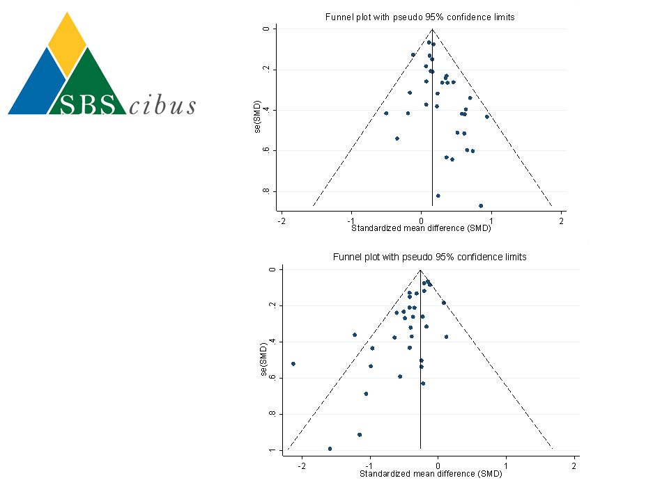
41. Funnel Plots

42. Publication bias +ve results more likely
To be published (publication bias)
To be published rapidly (time lag bias)
To be published in English (language bias)
To be published more than once (multiple publications bias)
To be cited by others (citation bias)

43. Sources of Bias Bias arising from the studies included in the review
Bias arising from the way the review is done
Publication bias is only one of the possible reasons for asymmetrical funnel plot
Funnel plot should been seen as a means of examining “small study effect”
We have quite a lot of evidence that these biases exist, so it is fair to assume that most systematic reviews will be subject to reporting bias to some extent.
If we accept that our review will almost certainly be subject to publication bias to some extent, we are left with the problem of estimating how big a problem it is in your review and what to do about it.

44. Publication bias Funnel plot Publication bias exists (asymmetrical)
Publication bias doesn’t exists (symmetrical)
For continuous data- Effect size plotted vs SE or sample size
For dichotomous data- LogOR or RR vs logSE or sample size
Fail Safe Number (F)
Z= (∑ ES/1.645)2-N: (where N= no of papers; ∑ ES is summed of effect size over all studies)-
for calculation of unpublished studies that would be required to negate the results of a significantly positive ES analysis.

46. Continuous data Funnel plot (continuous data)
metabias _ES _seES, egger
Contour-enhanced funnel plot
confunnel _ES _seES
Trim & Fill
metatrim _ES _seES, funnel print

47. Dichotomus data Funnel plot metabias _logES _selogES, egger
Contour-enhanced funnel plot
confunnel _logES _selogES
Trim & Fill
metatrim _logES _selogES, funnel print

48. Testing for funnel plot asymmetry-1
Cochrane group suggests that that tests for funnel plot asymmetry should be used in only a minority of meta-analyses (Ioannidis 2007)
Begg’s rank correlation test (adjusted rank correlation-low power)
This test is NOT recommended with any type of data
Eggers linear regression test (regression analysis-low power)
This test is mainly recommended for continuous data

49. Testing for funnel plot asymmetry-2
Peters (2006) & Harbord (2006) tests
These tests are suitable for dichotomous data with odds ratios
False-positive results may occur in the presence of substantial between-study heterogeneity
For dichotomous outcomes with risk ratios (RR) or risk differences (RD)
Firm guidance is not yet available

50. Correcting for publication bias
Trim and fill method (tail of the side of the funnel plot with smaller trials chopped off)
Fail safe N (required studies to overturn positive results)
Modelling for the probability of studies not published
Conclusion: there is no definite answer for assessing the presence of publication bias

51. Influence analysis
metaninf nt mean_t sd_t nc mean_c sd_c, label(namevar=study year) random cohen

52. References www.stata.com/support/faqs/stat/meta.html
Cochrane Collaboration Open learning material for reviewers (2002)
Higgins et al. (2001). BMJ 327:
Sterne et al. (2001). BMJ 323:
Whitehead A (2002). Meta-analysis of Controlled Clinical Trials