1. Drift models and polar field for cosmic rays propagation Stefano Della Torre 11th ICATPP, Como 5-9 october 2009

2. Outline Cosmic Rays propagation in different period/polarity Drift Models Solar Wind Heliosphere Conclusions

3. Modulation A>0 A<0 Tilt Angle from Wilcox Obs. Shikaze et al. 2007

4. Boella et. Al. 2001 Modulation There is a strong dependence of the modulation from the polarity of the field Variation between two consecutive minimum (it change the Field polarity) Rate of flux in two consecutive period with similar solar activity Boella et. Al. 2001

5. The Cosmic Rays propagation inside the heliosphere is described by the Parker equation U Cosmic Rays number density per unit interval of kinetic energy Cosmic Rays propagation Diffusion Small Scale Magnetic Field irregoularity Convection Presence of the solar wind moving out from the Sun Energetic Loss Due to adiabatic expansion of the solar wind Drift Large Scale structure of magnetic field (e.g. gradients)

6. Along the equatorial region, where the magnetic field invert his polarity, we have Neutral Sheet Drift Neutral Sheet Sheet with |B|=0 -> charge dependent -> Magnetic polarity dependent Magnetic Drift Drift This Effect is greater during solar minimum periods, when the Heliosferic Magnetic Field (HMF) have a regular topology, and vanishing during Solar Maxima due to chaotic behavior of the field line Potgieter et al. 1985

7. Neutral Sheet Coronal Magnetic Field lines at Solar minimum Activity The combination with the Solar Rotation cause a tilt of the Neutral Sheet; causing the so called “ballerina skirt” effect around the Eclittica Plane The amplitute of this oscillation is called Tilt Angle (  ) And it depends of Solar activity: e.g. minimum activity ->   10°, maximum activity ->  >75°

8. Neutral Sheet Drift Potgieter & Moraal (1985) Burger & Potgieter (1989) Wavy Neutral Sheet - Hattingh & Burger (1995) Ordinary Drift NS drift Transition Function that emulate the effect of a wavy neutral sheet 2D Approximation erer N S

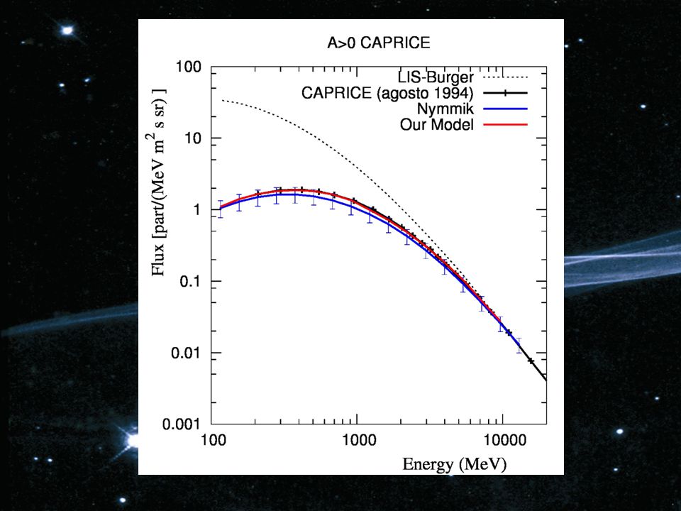
9. during solar Minimum AMS-01 (1998) CAPRICE (1994) Tilt Angle (  ) < 30°

10. Solar Wind High Solar Activity Low Solar Activity Ulysses measurement

11. Agreement with data

12. Modified Heliospheric Magnetic Field A We use a Simple Parker’s Field With a Polar modification as in Jokipii & Kòta 1989

13. Polar Cosmic Rays access reduced Agreement with data

14. A solar Magnetic perturbation generated TODAY on the Sun, will get the Heliopause in Dynamic view of HMF month We divide the heliosphere in 14 region, with previous solar condition each AMS-01 view of heliosphere A Cosmic Particle in average will remain  1 month into heliosphere

15. Agreement with data

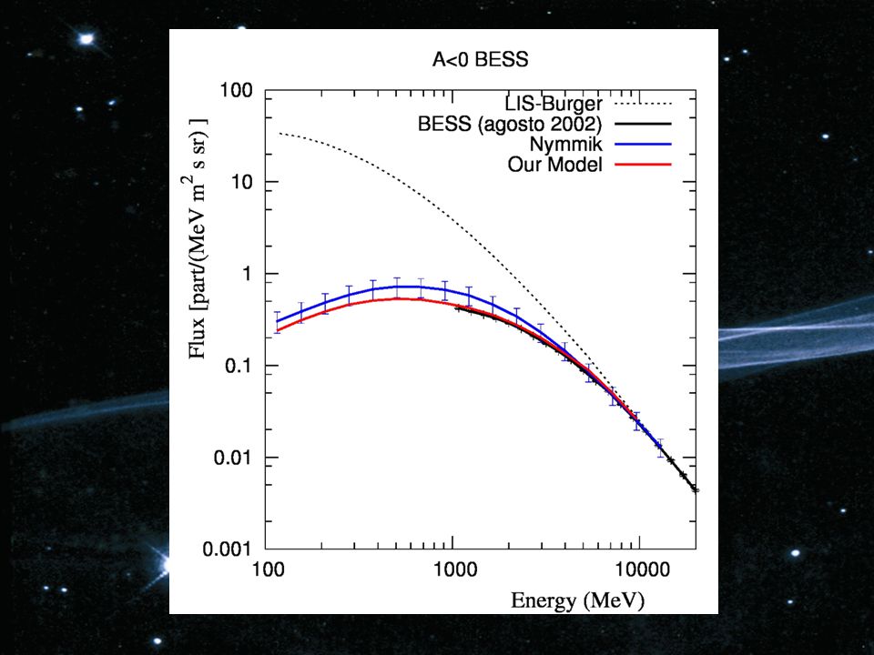
16. In all simulation presented we use PM model 30° A>0 A<0 BESS High Solar Activity AMS-01 Low Solar Activity IMAX Middle solar activity CAPRICE Low Solar Activity Experimental Data Nymmik  Empirical Model.  One parameter model: smoothed sunspot number in the months previous the oservations data.  For All Nuclei  Actually the ISO standard for space qualification.

21. Increase of precision compared with Nymmik model Our Average variance = 5% Nymmik Average variance = 16%

22. Conclusions We develop a 2D - MonteCarlo Stochastic program that reproduces Cosmic rays data in different solar periods using a dynamic view of HMF. We use a modified Magnetic field that reduces the drift contribute in polar regions. We find that during solar minimum both PM and WNS model reproduce data with confidence; increasing solar activity only PM model does that. The Solar wind latitudinal dependency is relevant in order to reproduce data

23. Thanks for Yours Attention Stefano.DellaTorre@mib.infn.it

24. The Cosmic Rays propagation inside the heliosphere is described by the Parker equation U Cosmic Rays number density per unit interval of kinetic energy Diffusive term Advective term (drift + Convection) Stochastic Approach The 2D - Parker equation is equivalent to a set of Stochastic Differential Equation

25. Proton created at 100 AU following the Local Interstellar Spectrum random walk propagation inside the heliosphere until they reach the lower energy admitted or they are scattered outside the heliosphere The passage trough the region of interest (e.g. 1 AU) is registered Stochastic Approach