1. Multiple Regression Analysis
Lecture 6
Multiple Regression Analysis

2. Objectives:
Explain and conduct multiple regression analysis in SPSS;
Interpret a multiple regression model; and
Check the assumptions and conditions of a multiple regression model
Lecture 6

3. The Multiple Regression Model
QTM1310/ Sharpe
For simple regression, the predicted value depends on only one predictor variable:
For multiple regression, we write the regression model with more predictor variables:
The Multiple Regression Model

4. Simple Regression Example
QTM1310/ Sharpe
The variation in Bedrooms accounts for only 21% of the variation in Price.
Perhaps the inclusion of another factor can account for a portion of the remaining variation.
Simple Regression Example 4

5. Multiple Regression Example
QTM1310/ Sharpe
Multiple Regression: Include Living Area as a predictor in the regression model.
Now the model accounts for 58% of the variation in Price.
Multiple Regression Example 5

6. Multiple Regression Coefficients
QTM1310/ Sharpe
NOTE: The meaning of the coefficients in multiple regression can be subtly different than in simple regression.
Price = – *Bedrooms *Living Area
Price drops with increasing bedrooms?
How can this be correct?
Multiple Regression Coefficients 6

7. Multiple Regression Coefficients
QTM1310/ Sharpe
In a multiple regression, each coefficient takes into account all the other predictor(s) in the model.
For houses with similar sized Living Areas:
more bedrooms means smaller bedrooms and/or smaller common living space.
Cramped rooms may decrease the value of a house.
Multiple Regression Coefficients 7

8. “Do more bedrooms tend to increase or decrease the price of a home?”
QTM1310/ Sharpe
So, what’s the correct answer to the question:
“Do more bedrooms tend to increase or decrease the price of a home?”
Correct answer:
“increase” if Bedrooms is the only predictor (“more bedrooms” may mean “bigger house”, after all!)
“decrease” if Bedrooms increases for fixed Living Area (“more bedrooms” may mean “smaller, more-cramped rooms”)
Multiple regression coefficients must be interpreted in terms of the other predictors in the model!
Multiple Regression Coefficients 8

9. QTM1310/ Sharpe
Ticket Prices
On a typical night about 15,000 people attend a Concert at Newcastle Entertainment Centre, paying an average price of more than $75 per ticket.
Data for most weeks of consider the variables Paid Attendance (thousands), # shows, Average Ticket Price ($) to predict Receipts ($million).
Consider the regression model for these variables.
Dependent variable is: Receipts($M)
R squared = 99.9% R squared (adjusted) = 99.9%
s = with 74 degrees of freedom
Source Sum of Squares df Mean Square F-ratio P-value
Regression <
Residual
Example 9

10. Example Ticket Prices Write the regression model for these variables.
QTM1310/ Sharpe
Ticket Prices
Write the regression model for these variables.
Interpret the coefficient of Paid Attendance.
Estimate receipts when paid attendance was 200,000 customer attending 30 shows at an average ticket price of $70.
Is this likely to be a good prediction? Why or why not?
Variable Coeff SE(Coeff) t-ratio P-value
Intercept – –
Paid Attend
# Shows Average
Ticket Price
Example 10

11. Example Ticket Prices Write the regression model for these variables.
QTM1310/ Sharpe
Ticket Prices
Write the regression model for these variables.
Interpret the coefficient of Paid Attendance. If the number of shows and ticket price are fixed, an increase of 1000 customers generates an average increase of $76,000 in receipts.
Estimate receipts when paid attendance was 200,000 customer attending 30 shows at an average ticket price of $70. $13.89 million
Is this likely to be a good prediction? Yes, R2 (adjusted) is 99.9% so this model explains most of the variability in Receipts.
Example 11

12. Assumptions and Conditions
QTM1310/ Sharpe
Linearity Assumption
Linearity Condition: Check each of the predictors.
Home Prices Example: Linearity Condition is well-satisfied for both Bedrooms and Living Area.
Assumptions and Conditions 12

13. Assumptions and Conditions
QTM1310/ Sharpe
Linearity Assumption
Linearity Condition: Also check the residual plot.
Home Prices Example: Linearity Condition is well-satisfied.
Assumptions and Conditions 13

14. Assumptions and Conditions
QTM1310/ Sharpe
Independence Assumption
As usual, there is no way to be sure the assumption is satisfied. But, think about how the data were collected to decide if the assumption is reasonable.
Randomization Condition: Does the data collection method introduce any bias?
Assumptions and Conditions 14

15. Assumptions and Conditions
QTM1310/ Sharpe
Equal Variance Assumption
Equal Spread Condition: The variability of the errors should be about the same for each predictor.
Use scatterplots to assess the Equal Spread Condition.
Residuals vs. Predicted Values: Home Prices
Assumptions and Conditions 15

16. Assumptions and Conditions
QTM1310/ Sharpe
Normality Assumption
Nearly Normal Condition: Check to see if the distribution of residuals is unimodal and symmetric.
Home Price Example: The ‘tails” of the distribution appear to be non-normal.
Assumptions and Conditions 16

17. Assumptions and Conditions
QTM1310/ Sharpe
Summary of Multiple Regression Model and Condition Checks:
Check Linearity Condition with a scatterplot for each predictor. If necessary, consider data re-expression.
If the Linearity Condition is satisfied, fit a multiple regression model to the data.
Find the residuals and predicted values.
Inspect a scatterplot of the residuals against the predicted values. Check for nonlinearity and non-uniform variation.
Assumptions and Conditions 17

18. Assumptions and Conditions
QTM1310/ Sharpe
Summary of Multiple Regression Model and Condition Checks:
Think about how the data were collected.
Do you expect the data to be independent?
Was suitable randomization utilized?
Are the data representative of a clearly identifiable population?
Is autocorrelation an issue?
Assumptions and Conditions 18

19. Assumptions and Conditions
QTM1310/ Sharpe
Summary of Multiple Regression Model and Condition Checks:
If the conditions check, feel free to interpret the regression model and use it for prediction.
Check the Nearly Normal Condition by inspecting a residual distribution histogram and a Normal plot. If the sample size is large, the Normality is less important for inference. Watch for skewness and outliers.
Assumptions and Conditions 19

20. QTM1310/ Sharpe
There are several hypothesis tests in multiple regression
Each is concerned with whether the underlying parameters (slopes and intercept) are actually zero.
The hypothesis for slope coefficients:
Test the hypothesis with an F-test (a generalization of the t-test to more than one predictor).
Testing the Model 20

21. Testing the Model The F-distribution has two degrees of freedom:
QTM1310/ Sharpe
The F-distribution has two degrees of freedom:
k, where k is the number of predictors
n – k – 1 , where n is the number of observations
The F-test is one-sided – bigger F-values mean smaller P-values.
If the null hypothesis is true, then F will be near 1.
Testing the Model 21

22. QTM1310/ Sharpe
If a multiple regression F-test leads to a rejection of the null hypothesis, then check the t-test statistic for each coefficient:
Note that the degrees of freedom for the t-test is n – k – 1.
Confidence interval:
Testing the Model 22

23. Testing the Model “Tricky” Parts of the t-tests:
QTM1310/ Sharpe
“Tricky” Parts of the t-tests:
SE’s are harder to compute (let technology do it!)
The meaning of a coefficient depends on the other predictors in the model (as we saw in the Home Price example).
If we fail to reject based on it’s t-test, it does not mean that xj has no linear relationship to y. Rather, it means that xj contributes nothing to modeling y after allowing for the other predictors.
Testing the Model 23

24. QTM1310/ Sharpe
In Multiple Regression, it looks like each tells us the effect of its associated predictor, xj.
BUT
The coefficient can be different from zero even when there is no correlation between y and xj.
It is even possible that the multiple regression slope changes sign when a new variable enters the regression.
Testing the Model 24

25. Example More Ticket Prices
QTM1310/ Sharpe
More Ticket Prices
On a typical night about 15,000 people attend a Concert at Newcastle Entertainment Centre, paying an average price of more than $75 per ticket.
Data for most weeks of consider the variables Paid Attendance (thousands), # shows, Average Ticket Price ($) to predict Receipts($million).
State hypothesis, the test statistic and p-value, and draw a conclusion for an F-test for the overall model.
Dependent variable is: Receipts($M)
R squared = 99.9% R squared (adjusted) = 99.9%
s = with 74 degrees of freedom
Source Sum of Squares df Mean Square F-ratio P-value
Regression <
Residual
Example 25

26. Example More Ticket Prices
QTM1310/ Sharpe
More Ticket Prices
State hypothesis for an F-test for the overall model.
State the test statistic and p-value. The F-statistic is the F-ratio = The p-value is <
Draw a conclusion. The p-value is small, so reject the null hypothesis. At least one of the predictors accounts for enough variation in y to be useful.
Example 26

27. Example More Ticket Prices
QTM1310/ Sharpe
More Ticket Prices
Since the F-ratio suggests that at least one variable is a useful predictor, determine which of the following variables contribute in the presence of the others. Recall the variables Paid Attendance (thousands), # shows, Average Ticket Price ($) to predict Receipts($million).
Variable Coeff SE(Coeff) t-ratio P-value
Intercept
Paid Attend
# Shows Average
Ticket Price
Example 27

28. Example More Ticket Prices
QTM1310/ Sharpe
More Ticket Prices
Since the F-ratio suggests that at least one variable is a useful predictor, determine which of the following variables contribute in the presence of the others.
Paid Attendance (p = ) and Average Ticket Price (p = ) both contribute, even when all other variables are in the model. # Shows however, is not significant (p = 0.116) and should be removed from the model.
Variable Coeff SE(Coeff) t-ratio P-value
Intercept
Paid Attend
# Shows Average
Ticket Price
Example 28

29. Example R2 in Multiple Regression:
QTM1310/ Sharpe
R2 in Multiple Regression:
fraction of the total variation in y accounted for by the model (all the predictor variables included)
R2 =
Adding new predictor variables to a model never decreases R2 and may increase it.
But each added variable increases the model complexity, which may not be desirable.
Adjusted R2 imposes a “penalty” on the correlation strength of larger models, depreciating their R2 values to account for an undesired increase in complexity.
Adjusted R2 permits a more equitable comparison between models of different sizes.
Example 29

30. Multiple Regression in SPSS Words
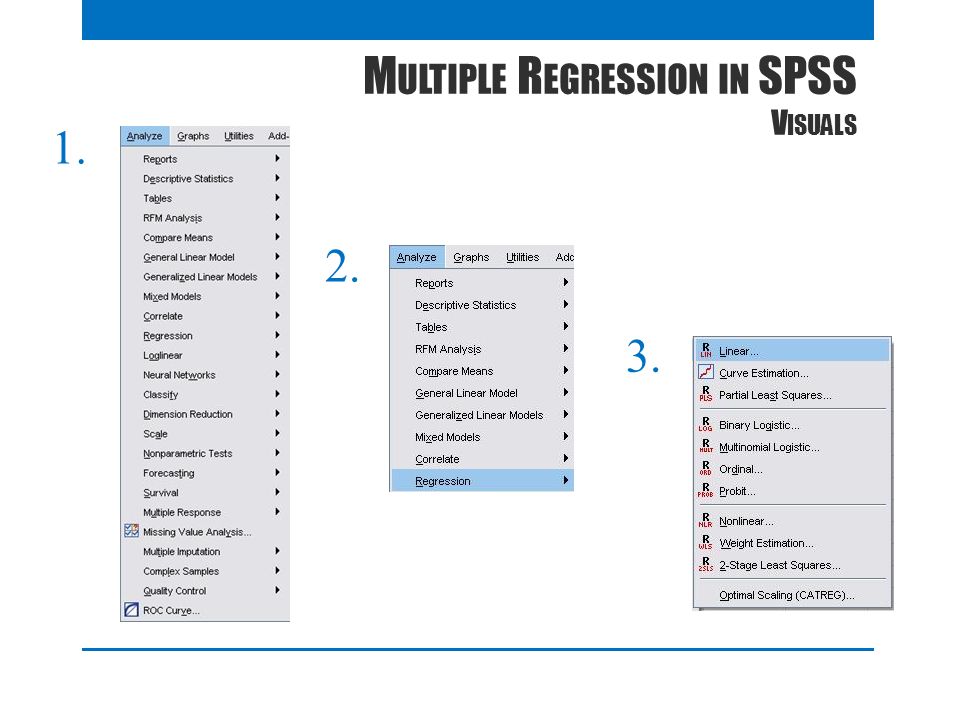
Analyze
Regression
Linear
Select the “Dependent Variable” - use the > button to move into the Dependent: box
Select the “Independent Variables” - use the > button to move into the Independent(s): box
Click Statistics
Select Descriptives

31. Multiple Regression in SPSS Visuals1. 2. 3.

32. Multiple Regression in SPSS Visuals5.
Use the > button to move variable into the Dependent: box
Use the > button to move variables into the Independent(s): box 6. 4.
Select Variables
Click Statistics 7. 8.
Select Descriptives

33. Multiple Regression in SPSS Output
R Square adjusted for the number of Independent variables and the sample size
Note: R Square is the
Coefficient of multiple determination. It shows the
strength of the association between the Dependent Variable (Y) and two or more Independent Variables (X’s) (From 0 to 1, usually reported as a percentage)
Is the relationship Significant?
That is, is it strong enough to indicate there is also a relationship in the population?
P value = < 0.05
Therefore, the relationship is significant
This tells us that 99.9% of the variation in Receipts can be explained by our linear regression model

34. Multiple Regression Output
Partial Regression Coefficients
These can be used to construct the regression equation for Receipts.
Receipts = a + b1X1 + b2X2 + b3X3 + … + bkXk
Receipts = *PaidAttendance *Shows *AvgTicketPrice
If we know the values for the three predictors we can use the regression equation to predict the Receipts value.

35. Multiple Regression Output
Testing the significance of the Regression Coefficients
The t and Sig t values given in the Coefficients table tell us which partial regression coefficients (slopes) differ significantly from zero.
In this example the variables that contribute significantly are:
PaidAttendance: t= , p=0.000
AvgTicketPrice: t=61.014, p=0.000
p-values < 0.05

36. Receipts = -18.320 + 0.076*PaidAttendance + 0.238*AvgTicketPrice
Model Which predictors are significant?
In this example the variables that contribute significantly are:
PaidAttendance: t= , p=0.000
AvgTicketPrice: t=61.014, p=0.000
p-values < 0.05
The regression equation can therefore be rewritten as:
Receipts = *PaidAttendance *AvgTicketPrice

37. Multiple Regression Output
Partial Regression Coefficients – INTERPRETATION
The partial regression coefficient for “AvgTicketPrice” might be interpreted:
If PaidAttendance is statistically controlled, an increase of 1 in AvgTicketPrice will INCREASE the predicted Receipts Value by

38. Multiple Regression Output
Standardised Regression Coefficients
Useful in assessing the relative importance of the predictors and comparing predictors across samples.
Are coefficients that have been adjusted so that the y intercept (constant) is zero and S.D is 1.
The most important predictor in this model is “PaidAttendance” (Beta = 0.955).

39. Multiple Regression Interpretation
Multiple Regression analysis was undertaken to determine the factors that contribute to Receipts (in millions) of the Newcastle Entertainment Centre. Results indicated that the number of paid attendees (t= , p=0.000) and the average ticket price (t=61.014, p=0.000) are significant predictors to this value. The most important predictor in the model was “PaidAttendance” (Beta = 0.955).
The regression models with the significant predictors is:
Receipts = *PaidAttendance *AvgTicketPrice

40. Multiple Regression Interpretation
Receipts = *PaidAttendance *AvgTicketPrice
If the average ticket price is statistically controlled (or fixed), an increase in 1000 paying customers will increase the Receipts value by $76,000.
If the number of paid attendees is statistically controlled, an increase of $1 in the average ticket price will generate an average increase in Receipts of $238.
This regression model explains 99.9% of the variation in the receipts generated for Newcastle Entertainment Centre. Therefore this is a good model as nearly all of the variability in Receipts is explained by this model.

41. QTM1310/ Sharpe
Don’t claim to “hold everything else constant” for a single individual. (For the predictors Age and Years of Education, it is impossible for an individual to get a year of education at constant age.)
Don’t interpret regression causally. Statistics assesses correlation, not causality.
Be cautious about interpreting a regression as predictive. That is, be alert for combinations of predictor values that take you outside the ranges of these predictors. 41

42. QTM1310/ Sharpe
Be careful when interpreting the signs of coefficients in a multiple regression. The sign of a variable can
change depending on which other predictors are in or out of the model. The truth is more subtle and requires that we understand the multiple regression model.
If a coefficient’s t-statistic is not significant, don’t interpret it at all.
Don’t fit a linear regression to data that aren’t straight. Usually, we are satisfied when plots of y against the x’s are straight enough. 42

43. Make sure the errors are nearly normal.
QTM1310/ Sharpe
Watch out for changing variance in the residuals. The most common check is a plot of the residuals against the predicted values.
Make sure the errors are nearly normal.
Watch out for high-influence points and outliers. 43

44. Fundamentals of Quantitative Analysis
Review
Fundamentals of Quantitative Analysis

45. Week 1: The Role, Collection and Presentation of Quantitative Data in the Business Decision Making Process
Week 2: Examining Data Characteristics: Descriptive Statistics and Data Screening
Week 3: Estimation and Hypothesis Testing
Week 4: Testing for Differences: One sample, Independent and Paired Sample t-tests and ANOVA
Week 5: Testing for Associations: Chi Square, Correlation and Simple Regression Analysis
Week 6: Multiple Regression Analysis
Lecture Plan

46. Objectives:
Explain the use of quantitative techniques in business;
Discuss the role of quantitative data analysis in the Business Decision Making Process;
Explain different sources of quantitative data and how it is collected;
Define and describe different types of data;
Recognise the potential for using different methods of data presentation in business;
Outline the major alternative methods of data presentation;
Select between the major alternative methods; and
Describe the limitations of data presentation methods.
Lecture 1

47. Lecture 2 Objectives: Describe and display categorical data;
Generate and interpret frequency tables, bar charts and pie charts;
Generate and interpret histograms to display the distribution of a quantitative variable;
Describe the shape, centre and spread of a distribution;
Compute descriptive statistics and select between mean/median and standard deviation / interquartile range; and
Explain data screening and its purpose, and be able to assess a distribution for normality.
Lecture 2

48. Objectives:
Formulate a null and alternate hypothesis for a question of interest;
Explain what a test statistic is;
Explain p-values;
Describe the reasoning of hypothesis testing;
Determine and check assumptions for the sampling distribution model;
Compare p-values to a pre-determined significance level to decide whether to reject the null hypothesis;
Recognise the value of estimating and reporting the effect size; and
Explain Type I and Type II errors when testing hypotheses.
Lecture 3

49. Objectives:
Recognise when to use a one sample t-test, independent samples t- test, paired samples t-test and ANOVA;
Explain and check the assumptions and conditions for each test;
Run and interpret a 'One sample t-test' to show a sample mean is different from some hypothesised value;
Run and interpret an ‘independent samples t-test’ to show the difference between two groups on one attribute;
Run and interpret a 'one-way ANOVA' to show the difference between more than two groups on one attribute; and
Run and interpret a ‘paired samples t-test’ to show the difference between two attributes as assessed by one sample.
Lecture 4

50. Objectives:
Recognise when a chi-square test of independence is appropriate;
Check the assumptions and corresponding conditions for a chi- square test of independence;
Run and interpret a chi-square test of independence;
Produce and explain a scatter plot to display the relationship between two quantitative variables;
Interpret the association between two quantitative variables using a Pearson's correlation coefficient;
Model a linear relationship with a least squares regression model;
Explain and Check the assumptions and conditions for inference about regression models; and
Examine the residuals from a linear model to assess the quality of the model.
Lecture 5

51. Objectives:
Explain and conduct multiple regression analysis in SPSS;
Interpret a multiple regression model; and
Check the assumptions and conditions of a multiple regression model
Lecture 6

52. Quantitative vs Qualitative Data
Quantitative vs Qualitative Data

53. End of Quantitative Model