1. The Cagan Model of Money and Prices
(Obstfeld-Rogoff)
Presented by: Emre Sakar
12/04/2013

2. Introduction In his paper, Cagan(1956) studied seven hyperinflations.
He defined hyperinflations as periods during which the price level of goods in terms of money rises at a rate averaging at least 50 percent per month.
This implies an annual inflation rate of almost 13,000 percent!
Cagan’s study encompassed episodes from Austria, Germany, Hungary, Poland and Russia after World War I, and from Greece and Hungary after World War II.

3. The Model Let M denote a country’s money supply and P its price level.
Cagan’s model for the demand of real money balances M/P is:
(1)
Where m= log of money balances held at the end of period t,
p=log P and ɳ is the semielasticity of demand for real balances with respect to expected inflation.
The analysis assumes rational expectations.
The equation (1) is a simplified form of the standard LM curve:
𝑀 𝑡 𝑑 𝑃 𝑡 =L( 𝑌 𝑡 , 𝑖 𝑡+1 ) (2)

4. Real money demand depends positively on aggregate real output 𝑌 𝑡 and negatively on the nominal interest rate 𝑖 𝑡+1
Cagan argued that during a hyperinflation, expected future inflation swamps all other influences on money demand.
Thus, one can ignore changes in real output Y and real interest rate r, which will not vary much compared with monetary factors.
The real interest rate links the nominal interest rate to inflation through Fisher parity equation:
1+ 𝑖 𝑡+1 =(1+ 𝑟 𝑡+1 ) 𝑃 𝑡+1 𝑃 𝑡 (3)
The nominal interest rate and expected inflation will move in lockstep if the real interest rate is constant, which explains Cagan’s simplification of making money demand a function of expected inflation.

5. Solving the Model
Having motivated Cagan’s money demand function, what are the relationship between money and the price level?
Assuming an exogenous money supply m, in equilibrium:
𝑚 𝑡 𝑑 = 𝑚 𝑡 , thus the monetary equilibrium condition:
(4)
So, we have an equation explaining price-level dynamics in terms of the money supply.

6. First, for the nonstochastic perfect foresight, ie,
First, for the nonstochastic perfect foresight, ie, by successive substitution of 𝑃 𝑡+2 ,𝑃 𝑡+3 ….. we get that:
(5)
we get that:
(6)
To check the reasonableness of solution (6), consider some simple cases:

7. Constant money supply:
Constant percentage growth rate:
Guessing that the price level is also growing at rate 𝜇, 𝑝 𝑡+1 − 𝑝 𝑡 = 𝜇. Substituting this guess in equations (5) and (6), we get again the same answer from both:

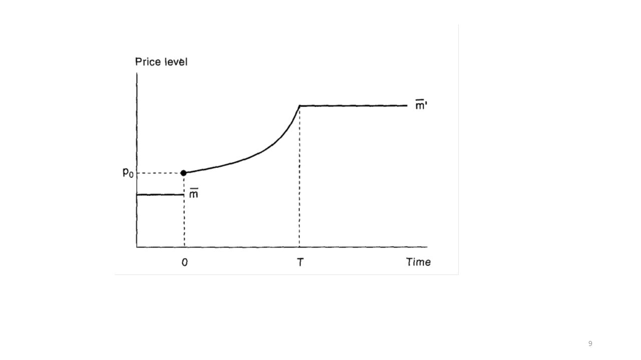
8. Solution (6) covers more general money supply processes.
Consider the effects of an unanticipated announcement on date t=0 that the money supply is going to rise sharply and permanently on a future date T. Specifically:
𝑚 𝑡 = 𝑚 , 𝑡<𝑇 & 𝑚 , 𝑡≥𝑇
Given this money supply path, eq. (6) gives the path of price level as:
𝑝 𝑡 = 𝑚 + 𝜂 1+𝜂 𝑇−𝑡 𝑚 − 𝑚 ,𝑡<𝑇 𝑝 𝑡 = 𝑚, 𝑡≥𝑇

10. The Stochastic Cagan Model
Given the linearity of the Cagan equation, extending its solution to a stochastic environment is straightforward. Under the no bubble assumption, we have that:
(8)
Suppose, for example, that the money supply process is governed by:
𝑚 𝑡 =𝜌 𝑚 𝑡−1 + ϵ 𝑡 , 0≤ 𝜌≤1, (9)
where ϵ 𝑡 is a serially uncorrelated white-noise money-supply shock such that 𝐸 𝑡 ϵ 𝑡+𝑠 =0 for s>0

11. The result is:
𝑝 𝑡 = 𝑚 𝑡 1+𝜂 𝑠=𝑡 ∞ 𝜂𝜌 1+𝜂 𝑠−𝑡 = 𝑚 𝑡 1+𝜂 1 1− 𝜂𝜌 1+𝜂 = 𝑚 𝑡 1+𝜂−𝜂𝜌
In the limiting case ρ=1 (in which money shocks are expected to be permanent, the solution reduces to 𝑝 𝑡 = 𝑚 𝑡 .

12. The Cagan Model in Continuous Time
Sometimes is easier to work in continuous time. In this case, the Cagan nonstochastic demand becomes:
(11)
where d(logP)/dt = 𝑃 /𝑃 is the anticipated inflation rate in continuous time. Using conventional differential equation methods, we get that:
(12)
Speculative bubbles are ruled out by setting the arbitrary constant 𝑏 0 𝑡𝑜 𝑧𝑒𝑟𝑜.

13. Seignorage
Definition: represents the real revenues a government acquires by using newly issued money to buy goods and nonmoney assets:
(13)
Most hyperinflations stem from the government’s need for seignorage revenue.
What are the limits to the real resources a government can obtain by printing money?

14. (14)
If higher money growth raises expected inflation, the demand for real balances M/P will fall, so that a rise in money growth does not necessarily augment seignorage revenues.
Finding the seignorage-revenue-maximizing rate of inflation is easy if we look only at constant rates of money growth:
(15)
Exponentiating Cagan’s perfect foresight demand, we get:
(16)

15. Substituting these equations into the seignorage equation (14) yields:
(17)
The FOC with respect to yields:
(18)
(19)
Cagan was surprised because, at least in a portion of each hyperinflation he studied, governments seem to put the money to grow at rates higher than the optimal one.

16. Cagan reasoned that if expectations of inflation are adaptive, and therefore backward-looking, then they may be a short-run benefit to government of temporarily exceeding the revenue- maximizing rate.
Even under forward-looking rational expectations, however, Cagan’s reasoning still points a subtle problem with steady state analysis of the seignorage-maximizing rate of inflation.
At t=0, suppose government announce that it will stick forever to the revenue-maximizing rate of money growth 1/ɳ.
If the public believes the government:
𝑀 𝑃 = [ 1+𝜂 𝜂 ] −𝜂 (20)
What if, at t=1, the government suddenly sets the money growth greater than 1/𝜂 , promising this will never happen again?
If the public believes, the government obtains higher period 1 revenues at no future costs.

17. If the public does not believe, the holdings of real balances will be below [ 1+𝜂 𝜂 ] −𝜂
Thus, unless a government can establish credibility for its money- growth announcement, its maximum seignorage revenue in reality may well be less than the maximum.

18. A Simple Model of Exchange Rates
A variant of Cagan’s model: a small open economy with exogenous real output and money demand given by:
(21)
i ≡ log(1+i)
p = logP
y = logY
Let 𝜀 be the nominal exchange rate (foreign in terms of home), and 𝑃 ∗ denote the world foreign-currency price of the consumption basket with home-currency price P.

19. Then, purchasing power parity (PPP) implies that:
(22)
(23)
Uncovered Interest Parity (UIP) holds when
(24)
An approximation in logs of UIP is:
(25)

20. Substituting the eq.(23) and (25) in eq. (21) gives:
(26)
And the solution for the exchange rate is:
(27)
Raising the path of the home money supply raises the domestic price level and forces ℯ up through the PPP mechanism.
Even though data do not support generally this model in non hyperinflation environment, this simple model yields one important insight that is preserved in more general frameworks:
The nominal exchange rate must be viewed as an asset price in the sense that it depends on expectations of future variables, just like other assets.

21. Example How to apply eq. (27) in practice.
Let y, p, and 𝑖 ∗ be constant with 𝜂 𝑖 ∗ -𝜙𝑦− 𝑝 ∗ =0, and suppose that money supply follows the process
𝑚 𝑡 − 𝑚 𝑡−1 =𝜌 𝑚 𝑡−1 − 𝑚 𝑡−2 + 𝜖 𝑡 , ≤ 𝜌 ≤1 (28)
where 𝜖 is a seriallly uncorrelated mean-zero shock such that 𝐸 𝑡−1 𝜖 𝑡 =0
To evaluate the solution (27), lead by one period, take date t expectations of both sides, and then subtract the original equation:
𝐸 𝑡 𝑒 𝑡+1 − 𝑒 𝑡 = 1 1+𝜂 𝑠=𝑡 ∞ 𝜂 1+𝜂 𝑠−𝑡 𝐸 𝑡 𝑚 𝑠+1 − 𝑚 𝑠 (29)
Substituting eq. (28) into (29) yields:

22. 𝐸 𝑡 𝑒 𝑡+1 − 𝑒 𝑡 = 𝜌 1+𝜂−𝜂𝜌 ( 𝑚 𝑡 − 𝑚 𝑡−1 ) (30)
Substituting this expression into eq. (26) yields the solution for the exchange rate:
𝑒 𝑡 = 𝑚 𝑡 + 𝜂𝜌 1+𝜂−𝜂𝜌 ( 𝑚 𝑡 − 𝑚 𝑡−1 ) (31)
This equation shows that an unanticipated shock to 𝑚 𝑡 may have two impacts:
1. It always raises the exchange rate directly by raising the current
nominal money supply.
2. When 𝜌>0, it also raises expectations of future money growth,
thereby pushing the exchange rate even higher.
Thus, this simple monetary-model provides one story of how
instability in the money supply could lead to proportionally greater
variability in the exchange rate.

23. Thank you!