1. An Introduction to MATLAB® Dr M Ali Ahmadi-Pajouh KN Toosi University

2. MATLAB= Matrix + Laboratory Usage : –Math and computation Algorithm – development Data acquisition Modeling simulation, and prototyping –Data analysis exploration, and visualization –Scientific and engineering graphics –Application development, including graphical user interface building –…

3. Development Environment

4. Desktop Tools Command Window

5. Desktop Tools Start = easy access to tools, demos, and documentation.

6. Current Directory Browser file you want to run must either be in the current directory or on the search path

7. Workspace Browser

8. Editor/Debugger M-files are programs you write to run MATLAB functions.

9. Matrix To enter a matrix, simply type in the Command Window: A = [16 3 2 13; 5 10 11 8; 9 6 7 12; 4 15 14 1] MATLAB displays the matrix you just entered. A = 16 3 2 13 5 10 11 8 9 6 7 12 4 15 14 1

10. Transpose So A' produces ans = 16 5 9 4 3 10 6 15 2 11 7 14 13 8 12 1 A = 16 3 2 13 5 10 11 8 9 6 7 12 4 15 14 1

11. Diagonal Elements diag(A) produces ans = 16 10 7 1 A = 16 3 2 13 5 10 11 8 9 6 7 12 4 15 14 1

12. Assigning a new Value to an Element X(4,4) = 17 X = 16 3 2 13 5 10 11 8 9 6 7 12 4 15 14 17 A = 16 3 2 13 5 10 11 8 9 6 7 12 4 15 14 1

13. Storing an Element >>t = A(4,3) t= 14 A = 16 3 2 13 5 10 11 8 9 6 7 12 4 15 14 1

14. The Colon Operator The expression 1:10 is a row vector containing the integers from 1 to 10: 1 2 3 4 5 6 7 8 9 10 To obtain nonunit spacing, specify an increment. For example, 100:-7:50 is 100 93 86 79 72 65 58 51

15. The Colon Operator Subscript expressions involving colons refer to portions of a matrix. A(1:k, j) is the first k elements of the jth column of A colon by itself refers to all the elements in a row or column of a matrix. A( :, 1) A( 2, :)

16. Some Other Good Operations To swap the two middle columns. A = B(:,[1 3 2 4]) To Erase an entire row or column A(1,:)=[] To Add a new row or column B=[A;[1 2 1 5]]

17. Variable MATLAB does not require any type declarations or dimension statements. the variable already exists, MATLAB changes its contents MATLAB is case sensitive To view the matrix assigned to any variable, simply enter the variable name

18. Format All computations in MATLAB are done in double precision. FORMAT may be used to switch between different output display formats as follows: FORMAT Default. Same as SHORT. FORMAT SHORT Scaled fixed point format with 5 digits FORMAT LONG Scaled fixed point format with 15 digits FORMAT HEX Hexadecimal format.

19. Cell Arrays They are multidimensional arrays whose elements are copies of other arrays. Example: >>C = {A sum(A) prod(prod(A))} ans= C = [4x4 double] [1x4 double] [20922789888000] If you subsequently change A, nothing happens to C

20. useful constants. Pi3.14159265... iImaginary unit sqrt(-1) jSame as i epsFloating-point relative precision 2 -52 realmin Smallest floating-point number, 2 -1022 realmax Largest floating-point number, 2 -21023 InfInfinity NaNNot-a-number

21. Operations + Addition - Subtraction * Multiplication / Division \ Left division (described in "Matrices and Linear Algebra" in the MATLAB documentation) ^ Power Complex conjugate transpose ( ) Specify evaluation order

22. Example [1+j 2+2*j]' ans = 1.0000 - 1.0000i 2.0000 - 2.0000i >>3/10 ans = 0.3000 >> 10\3 ans = 0.3000

23. rho = (1+sqrt(5))/2 rho = 1.6180 a = abs(3+4i) a = 5 z = sqrt(besselk(4/3,rho-i)) z = 0.3730+ 0.3214i huge = exp(log(realmax)) huge = 1.7977e+308 toobig = pi*huge toobig = Inf

24. Generating Matrices Z = zeros(2,4) Z = 0 0 0 0 F = 5*ones(3,3) F = 5 5 5 N = fix(10*rand(1,10)) N = 4 9 4 4 8 5 2 6 8 0 R = randn(4,4) R = 1.0668 0.2944 -0.6918 -1.4410 0.0593 -1.3362 0.8580 0.5711 -0.0956 0.7143 1.2540 -0.3999 -0.8323 1.6236 -1.5937 0.6900

25. Some Useful functions A' d = det(A) X = inv(A) e = eig(A) poly(A) sin(x) sinh(x) asin(x)

26. Array Operators + Addition - Subtraction.* Element-by-element multiplication./ Element-by-element division.\Element-by-element left division.^Element-by-element power.' Unconjugated array transpose

27. Example n = (0:9)'; Then pows = [n n.^2 2.^n] builds a table of squares and powers of 2. pows = 0 0 1 1 1 2 2 4 4 3 9 8 4 16 16 5 25 32 6 36 64 7 49 128 8 64 256 9 81 512

28. >> a=[1 2 3 4] >> b=[1 2 3 4]' >> a*b ans = 30 >> b*a ans = 1 2 3 4 2 4 6 8 3 6 9 12 4 8 12 16 >> a.*b' ans = 1 4 9 16

29. B = 7.5 -5.5 -6.5 4.5 -3.5 1.5 2.5 -0.5 0.5 -2.5 -1.5 3.5 -4.5 6.5 5.5 -7.5 >>B(1:2,2:3) = 0 B = 7.5 0 0 4.5 -3.5 0 0 -0.5 0.5 -2.5 -1.5 3.5 -4.5 6.5 5.5 -7.5

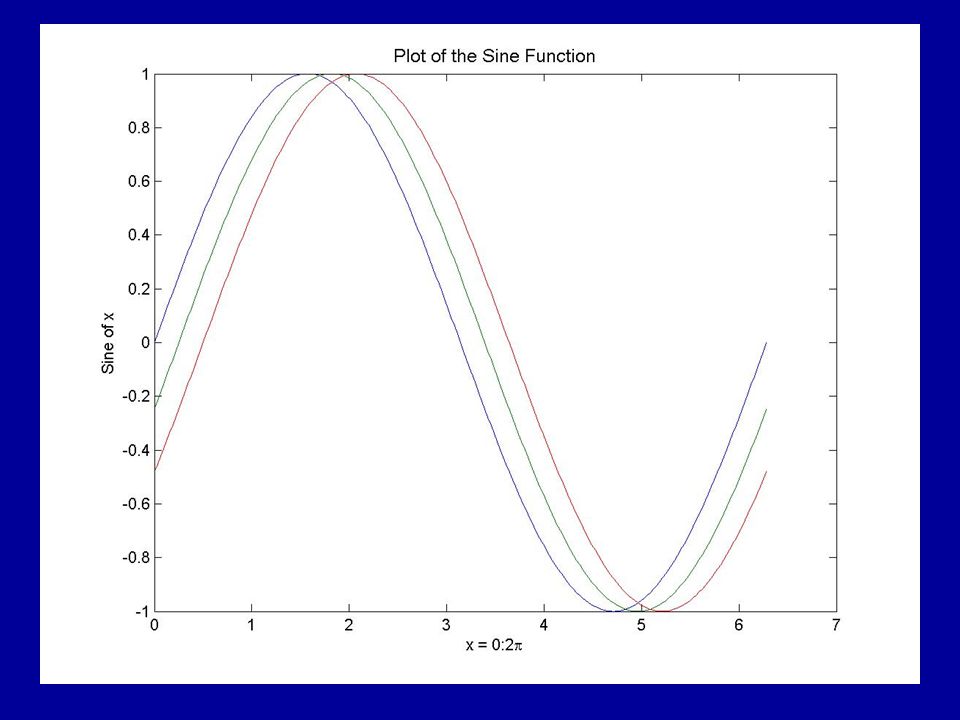
30. Geraphics PLOT: x = 0:pi/100:2*pi; y = sin(x); plot(x,y) xlabel('x = 0:2\pi') ylabel('Sine of x') title('Plot of the Sine Function','FontSize',12)

32. Multiple Data Sets in One Graph y2 = sin(x-.25); y3 = sin(x-.5); plot(x,y,x,y2,x,y3)

34. Colors 'c= cyan 'm=magenta 'y= yellow 'r= red 'g= green 'b= blue 'w= white 'k=black

35. plot(x,y,'ks')

36. plot(x,y,'k>')

37. plot(x,y,'r:+')

38. This example plots the data twice using a different number of points for the dotted line and marker plots. x1 = 0:pi/100:2*pi; x2 = 0:pi/10:2*pi; plot(x1,sin(x1),'r:',x2,sin(x2),'r+')

40. Complex Data When the arguments to plot are complex, the imaginary part is ignored For the special case of giving the plot a single complex argument, the command is a shortcut for a plot of the real part versus the imaginary part. Therefore, plot(Z)where Z is a complex vector or matrix, is equivalent to plot(real(Z),imag(Z))

41. Adding Plots to an Existing Graph hold on Example: [x,y,z] = peaks; contour(x,y,z,20,'k') hold on pcolor(x,y,z) shading interp hold off

42. Multiple Plots in One Figure subplot(m,n,p) Example: t = 0:pi/10:2*pi; [X,Y,Z] = cylinder(4*cos(t)); subplot(2,2,1); mesh(X) subplot(2,2,2); mesh(Y) subplot(2,2,3); mesh(Z) subplot(2,2,4); mesh(X,Y,Z)

44. Setting Axis axis([xmin xmax ymin ymax zmin zmax]) axis auto axis on axis off grid on grid off

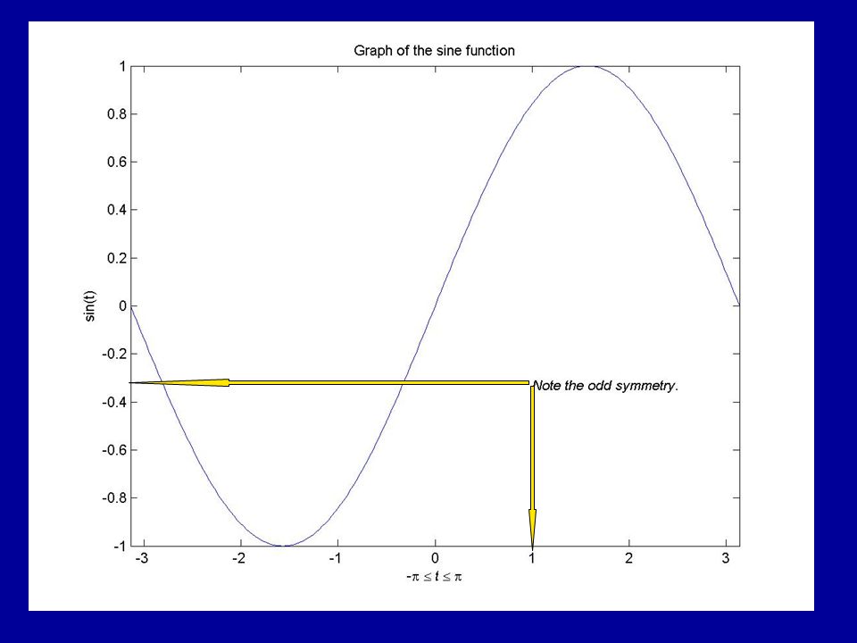
45. Example t = -pi:pi/100:pi; y = sin(t); plot(t,y) axis([-pi pi -1 1]) xlabel('-\pi \leq {\itt} \leq \pi') ylabel('sin(t)') title('Graph of the sine function') text(1,-1/3,'{\itNote the odd symmetry.}')

47. Mesh and Surface Plots Mesh (x,y,z) produces wireframe surfaces that color only the lines connecting the defining points. surf (x,y,z) displays both the connecting lines and the faces of the surface in color.

48. [X,Y] = meshgrid(-8:.5:8); R = sqrt(X.^2 + Y.^2) + eps; Z = sin(R)./R; mesh(X,Y,Z,'EdgeColor','black')

49. transparency hidden off

50. Surf Example surf(X,Y,Z) colormap hsv colorbar

51. View view(az,el) view([az,el])

52. Surface Plots with Lighting surf(X,Y,Z,'FaceColor','red','EdgeColor','none'); camlight left; lighting phong view(-15,65)

53. Flow Control if rem(n,2) ~= 0 ……………. elseif rem(n,4) ~= 0 ……………… else ………………. end

54. Important! when A and B are matrices, A == B does not test if they are equal, it tests where they are equal; the result is another matrix of 0's and 1's showing element-by-element equality. Solution: if isequal(A,B),...

55. Some Other Helpful Functions Isequal(A,B,…): Determine if arrays are numerically equal Isempty(A): Determine if item is an empty array isequalwithequalnans(A,B,...): Determine if arrays are numerically equal, treating NaNs as equal ismember(A,S): Detect members of a specific set isnumeric(A): Returns logical true (1) if A is a numeric array and logical false (0) otherwise.

56. Some Other Helpful Functions isprime(A): returns an array the same size as A containing logical true (1) for the elements of A which are prime. isreal(A): returns logical false (0) if any element of array A has an imaginary component, even if the value of that component is 0. ischar(A): ischar(A) returns logical true (1) if A is a character array and logical false (0) otherwise.

57. all(A): If A is a vector, all(A) returns logical true (1) if all of the elements are nonzero, and returns logical false (0) if one or more elements are zero. If A is a matrix, all(A) treats the columns of A as vectors, returning a row vector of 1s and 0s.

58. B = any(A): If A is a vector, any(A) returns logical true (1) if any of the elements of A are nonzero, and returns logical false (0) if all the elements are zero. If A is a matrix, any(A) treats the columns of A as vectors, returning a row vector of 1s and 0s.

59. Example: >>A = [0.53 0.67 0.01 0.38 0.07 0.42 0.69] B = (A < 0.5) Ans= 0 0 1 1 1 1 0 >>all(B) Ans=0 >>any(B) Ans=1 تابع ماتريسي

60. Relational Operators A < B A > B A <= B A >= B A == B A ~= B EXAMPLE: >>X = 5*ones(3,3); >>X >= [1 2 3; 4 5 6; 7 8 10]; ans = 1 1 1 1 1 0 0 0 0

61. Logical Operators The precedence for the logical operators The truth table The second operand is evaluated only when the result is not fully determined by the first operand.

62. Example >>u = [0 0 1 1 0 1]; >>v = [0 1 1 0 0 1]; >>u | v ans = 0 1 1 1 0 1 to avoid generating a warning when the divisor, b, is zero. x = (b ~= 0) && (a/b > 18.5) Logical Operation on Elements Short Circuit and

63. Flow Control switch (rem(n,4)==0) + (rem(n,2)==0) case 0 ……………………. case 1 ……………………. case 2 ……………………… otherwise error('This is impossible') end

64. Important! Unlike the C language switch statement, MATLAB switch does not fall through. If the first case statement is true, the other case statements do not execute. So, break statements are not required.

65. Flow Control for variable = scalar1 : step : scalar2 statement 1... statement n end Example:a = zeros(k,k) % Preallocate matrix for m = 1:k for n = 1:k a(m,n) = 1/(m+n -1); end

66. while expression statements End The statements are executed while the real part of expression has all nonzero elements.

67. Two Useful Functions for Loops Continue: Passes control to the next iteration of for or while loop Break: statement lets you exit early from a for or while loop.

68. Characters and Numbers To define a string: >>s = 'Hello characters are stored as numbers, but not in floating-point format. To see the characters as numbers: >>a = double(s) a = 72 101 108 108 111 To reverses the conversion: >>s = char(a)

69. M-files: 1.Scripts, which do not accept input arguments or return output arguments. They operate on data in the workspace. 2.Functions, which can accept input arguments and return output arguments. Internal variables are local to the function.

70. Functions 1.Checks to see if the name is a variable. 2.Checks to see if the name is an internal function (eig, sin) that was not overloaded. 3.Checks to see if the name is a local function (local in sense of multifunction file). 4.Checks to see if the name is a function in a private directory. 5.Locates any and all occurrences of function in method directories and on the path. Order is of no importance. At execution, MATLAB: 6.Checks to see if the name is wired to a specific function (2, 3, & 4 above) 7.Uses precedence rules to determine which instance from 5 above to call (we may default to an internal MATLAB function). Constructors have higher precedence than anything else.

71. Functions nargin and nargout indicate how many input or output arguments, respectively, a user has supplied. if nargout == 0 plot(x,y) else x0 = x; y0 = y; end if nargin < 5, subdiv = 20; end if nargin < 4, angl = 10; end if nargin < 3, npts = 25; end

72. function [x0,y0] = myplot(fname,lims,npts,angl,subdiv) % MYPLOT Plot a function. % MYPLOT(fname,lims,npts,angl,subdiv) % The first two input arguments are % required; the other three have default values.... if nargin < 5, subdiv = 20; end if nargin < 4, angl = 10; end if nargin < 3, npts = 25; end... if nargout == 0 plot(x,y) else x0 = x; y0 = y; end function h = falling(t) global GRAVITY h = 1/2*GRAVITY*t.^2;

73. A review on Mathematical Functions Binary additionA+Bplus(A,B) Unary plus +Auplus(A)Binary Subtraction A-Bminus(A,B) Unary minus-Auminus(A)Matrix MultiplicationA*Bmtimes(A,B)Array-wise Multiplication A.*Btimes(A,B)Matrix right DivisionA/Bmrdivide(A,B)Array-wise right DivisionA./Brdivide(A,B)Matrix left DivisionA\Bmldivide(A,B)Array-wise left DivisionA.\Bldivide(A,B)Matrix PowerA^Bmpower(A,B)Array-wise PowerA.^Bpower(A,B)Complex TransposeActranspose(A)Matrix TransposeA.transpose(A)