Download presentation
Presentation is loading. Please wait.

1
Discrete Choice Modeling
William Greene Stern School of Business New York University Lab Sessions

2
Discrete Choice, Multinomial Logit Model
Lab Session 8 Discrete Choice, Multinomial Logit Model

3
Observed Data Types of Data Attributes and Characteristics
Individual choice Market shares Frequencies Ranks Attributes and Characteristics Choice Settings Cross section Repeated measurement (panel data)
")
4
Data for Multinomial Choice
Line MODE TRAVEL INVC INVT TTME GC HINC 1 AIR 2 TRAIN 3 BUS 4 CAR 5 AIR 6 TRAIN 7 BUS 8 CAR 321 AIR 322 TRAIN 323 BUS 324 CAR 325 AIR 326 TRAIN 327 BUS 328 CAR

5
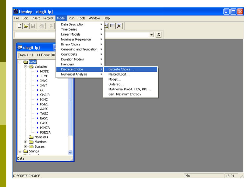
Using NLOGIT To Fit the Model
Start program Load CLOGIT.LPJ project Use command builder dialog box or Use typed commands in editor

7
Specification of Choice Variable

8
Specification of Utility Functions
Copy the variable names from the list at the right into the appropriate window at the left, then press Run

9
Submit Command from Editor
Type commands in editor Highlight by dragging mouse Press GO button

10
Command Structure Generic For this application
CLOGIT (or NLOGIT) ; Lhs = choice variable ; Choices = list of labels for the J choices ; RHS = list of attributes that vary by choice ; RH2 = list of attributes that do not vary by choice $ For this application CLOGIT (or NLOGIT) ; Lhs = MODE ; Choices = Air, Train, Bus, Car ; RHS = TTME,INVC,INVT,GC ; RH2 = ONE, HINC $
 ; Lhs = choice variable. ; Choices = list of labels for the J choices. ; RHS = list of attributes that vary by choice. ; RH2 = list of attributes that do not vary by choice $ For this application. CLOGIT (or NLOGIT) ; Lhs = MODE. ; Choices = Air, Train, Bus, Car. ; RHS = TTME,INVC,INVT,GC. ; RH2 = ONE, HINC $")
11
Output Window Note: coef. on GC has the wrong sign!

12
Effects of Changes in Attributes on Probabilities
Partial Effects: Effect of a change in attribute “k” of alternative “m” on the probability that choice “j” will be made is Proportional changes: Elasticities Note the elasticity is the same for all choices “j.” (IIA)
")
13
Elasticities for CLOGIT
Request: ;Effects: attribute (choices where changes ) ; Effects: INVT(*) (INVT changes in all choices) | Elasticity averaged over observations.| | Attribute is INVT in choice AIR | | Effects on probabilities of all choices in model: | | * = Direct Elasticity effect of the attribute. | | Mean St.Dev | | * Choice=AIR | | Choice=TRAIN | | Choice=BUS | | Choice=CAR | | Attribute is INVT in choice TRAIN | | Choice=AIR | | * Choice=TRAIN | | Choice=BUS | | Choice=CAR | | Attribute is INVT in choice BUS | | Choice=AIR | | Choice=TRAIN | | * Choice=BUS | | Choice=CAR | | Attribute is INVT in choice CAR | | Choice=AIR | | Choice=TRAIN | | Choice=BUS | | * Choice=CAR | Own effect Cross effects Note the effect of IIA on the cross effects.
 ; Effects: INVT(*) (INVT changes in all choices) | Elasticity averaged over observations.| | Attribute is INVT in choice AIR | | Effects on probabilities of all choices in model: | | * = Direct Elasticity effect of the attribute. | | Mean St.Dev | | * Choice=AIR | | Choice=TRAIN | | Choice=BUS | | Choice=CAR | | Attribute is INVT in choice TRAIN | | Choice=AIR | | * Choice=TRAIN | | Choice=BUS | | Choice=CAR | | Attribute is INVT in choice BUS | | Choice=AIR | | Choice=TRAIN | | * Choice=BUS | | Choice=CAR | | Attribute is INVT in choice CAR | | Choice=AIR | | Choice=TRAIN | | Choice=BUS | | * Choice=CAR | Own effect. Cross effects. Note the effect of IIA on the cross effects.")
14
Other Useful Options ; Describe for descriptive by statistics, by alternative ; Crosstab for crosstabulations of actuals and predicted ; List for listing of outcomes and predictions ; Prob = name to create a new variable with fitted probabilities ; IVB = log sum, inclusive value. New variable

15
Analyzing Behavior of Market Shares
Scenario: What happens to the number of people how make specific choices if a particular attribute changes in a specified way? Fit the model first, then using the identical model setup, add ; Simulation = list of choices to be analyzed ; Scenario = Attribute (in choices) = type of change For the CLOGIT application, for example ; Simulation = * ? This is ALL choices ; Scenario: INVC(car)=[*]1.25$ INVC rises by 25%
 = type of change. For the CLOGIT application, for example. ; Simulation = * This is ALL choices. ; Scenario: INVC(car)=[*]1.25$ INVC rises by 25%")
16
More Complicated Model Simulation
In vehicle cost of CAR rises by 25% Market is limited to ground (Train, Bus, Car) NLOGIT ; Lhs = Mode ; Choices = Air,Train,Bus,Car ; Rhs = TTME,INVC,INVT,GC ; Rh2 = One ,Hinc ; Simulation = TRAIN,BUS,CAR ; Scenario: INVC(car)=[*]1.25$
 NLOGIT ; Lhs = Mode. ; Choices = Air,Train,Bus,Car. ; Rhs = TTME,INVC,INVT,GC. ; Rh2 = One ,Hinc. ; Simulation = TRAIN,BUS,CAR. ; Scenario: INVC(car)=[*]1.25$")
17
Model Simulation In vehicle cost of CAR rises by 25%
|Simulations of Probability Model | |Model: Discrete Choice (One Level) Model | |Simulated choice set may be a subset of the choices. | |Number of individuals is the probability times the | |number of observations in the simulated sample | |Column totals may be affected by rounding error | |The model used was simulated with observations.| Specification of scenario 1 is: Attribute Alternatives affected Change type Value INVC CAR Scale base by value The simulator located observations for this scenario. Simulated Probabilities (shares) for this scenario: |Choice | Base | Scenario | Scenario - Base | | |%Share Number |%Share Number |ChgShare ChgNumber| |TRAIN | | | % | |BUS | | | % | |CAR | | | % | |Total | | | % | Changes in the predicted market shares when INVC_CAR changes
 Model | |Simulated choice set may be a subset of the choices. | |Number of individuals is the probability times the | |number of observations in the simulated sample. | |Column totals may be affected by rounding error. | |The model used was simulated with 210 observations.| Specification of scenario 1 is: Attribute Alternatives affected Change type Value INVC CAR Scale base by value The simulator located 209 observations for this scenario. Simulated Probabilities (shares) for this scenario: |Choice | Base | Scenario | Scenario - Base | | |%Share Number |%Share Number |ChgShare ChgNumber| |TRAIN | | | 3.390% 7 | |BUS | | | 2.755% 5 | |CAR | | | % -13 | |Total | | | .000% -1 | Changes in the predicted market shares when INVC_CAR changes.")
18
Compound Scenario: INVC(Car) falls by 10%, TTME (Air,Train) rises by 25% (at the same time).
|Simulations of Probability Model | |Model: Discrete Choice (One Level) Model | |Simulated choice set may be a subset of the choices. | |Number of individuals is the probability times the | |number of observations in the simulated sample | |Column totals may be affected by rounding error | |The model used was simulated with observations.| Specification of scenario 1 is: Attribute Alternatives affected Change type Value INVC CAR Scale base by value TTME AIR TRAIN Scale base by value The simulator located observations for this scenario. Simulated Probabilities (shares) for this scenario: |Choice | Base | Scenario | Scenario - Base | | |%Share Number |%Share Number |ChgShare ChgNumber| |AIR | | | % | |TRAIN | | | % | |BUS | | | % | |CAR | | | % | |Total | | | % | ;simulation=* ; scenario: INVC(car)=[*]0.9 / TTME(air,train)=[*]1.25
 Model | |Simulated choice set may be a subset of the choices. | |Number of individuals is the probability times the | |number of observations in the simulated sample. | |Column totals may be affected by rounding error. | |The model used was simulated with 210 observations.| Specification of scenario 1 is: Attribute Alternatives affected Change type Value INVC CAR Scale base by value TTME AIR TRAIN Scale base by value The simulator located 209 observations for this scenario. Simulated Probabilities (shares) for this scenario: |Choice | Base | Scenario | Scenario - Base | | |%Share Number |%Share Number |ChgShare ChgNumber| |AIR | | | % -23 | |TRAIN | | | % -15 | |BUS | | | 4.209% 9 | |CAR | | | % 29 | |Total | | | .000% 0 | ;simulation=* ; scenario: INVC(car)=[*]0.9 / TTME(air,train)=[*]1.25.")
19
Choice Based Sampling Over/Underrepresenting alternatives in the data set Biases in parameter estimates Biases in estimated variances Weighted log likelihood, weight = j / Fj for all i. Fixup of covariance matrix ; Choices = list of names / list of true proportions $ ; Choices = Air,Train,Bus,Car / 0.14, 0.13, 0.09, 0.64 Choice Air Train Bus Car True 0.14 0.13 0.09 0.64 Sample 0.28 0.30

20
Choice Based Sampling Estimators
Variable| Coefficient Standard Error b/St.Er. P[|Z|>z] Unweighted TTME| *** INVC| *** INVT| *** GC| *** A_AIR| *** AIR_HIN1| A_TRAIN| *** TRA_HIN2| *** A_BUS| *** BUS_HIN3| Weighted TTME| *** INVC| *** INVT| *** GC| *** A_AIR| *** AIR_HIN1| A_TRAIN| *** TRA_HIN2| *** A_BUS| *** BUS_HIN3|

21
Changes in Estimated Elasticities
| Unweighted | | Elasticity averaged over observations.| | Attribute is INVC in choice CAR | | Effects on probabilities of all choices in model: | | * = Direct Elasticity effect of the attribute. | | Mean St.Dev | | Choice=AIR | | Choice=TRAIN | | Choice=BUS | | * Choice=CAR | | Weighted | | Choice=AIR | | Choice=TRAIN | | Choice=BUS | | * Choice=CAR |

22
Testing IIA vs. AIR Choice
? No alternative constants in the model NLOGIT ; Lhs = Mode ; Choices = Air,Train,Bus,Car ; Rhs = TTME,INVC,INVT,GC$ ; Rhs = TTME,INVC,INVT,GC ; IAS = Air $

23
Testing IIA – Dealing with Constants
With ASCs in the model, the covariance matrix becomes singular because the constant for AIR is always zero within the reduced sample. Do the test against the other coefficients. NLOGIT ; Lhs = Mode ; Choices = Air,Train,Bus,Car ; Rhs = TTME,INVC,INVT,GC,One$ MATRIX ; Bair = b(1:4) ; Vair = Varb(1:4,1:4) $ ; Rhs = TTME,INVC,INVT,GC,One ; IAS = Air$ MATRIX ; BNoair=b(1:4) ; VNoair = Varb(1:4,1:4) $ MATRIX ; Db = BNoair-BAir ; Dv = VNoair - Vair $ MATRIX ; List ; H = Db'<Dv>Db $
 ; Vair = Varb(1:4,1:4) $ ; Rhs = TTME,INVC,INVT,GC,One. ; IAS = Air$ MATRIX ; BNoair=b(1:4) ; VNoair = Varb(1:4,1:4) $ MATRIX ; Db = BNoair-BAir ; Dv = VNoair - Vair $ MATRIX ; List ; H = Db <Dv>Db $")
24
Nested Logit Models Extensions of the MNL
Lab Session 8 Part 2 Nested Logit Models Extensions of the MNL

25
Using NLOGIT To Fit the Model
Start program Load CLOGIT.LPJ project Specify trees with :TREE = name1(alt1,alt2…), name2(alt…. ),… “Names” are optional names for branches.
, name2(alt…. ),… Names are optional names for branches.")
26
Nested Logit Model ? Load the CLOGIT data ?
? (1) A simple nested logit model NLOGIT ; Lhs = Mode ; RHS = GC, TTME, INVT ; RH2 = ONE ; Choices = Air,Train,Bus,Car ; Tree = Private (Air,Car) , Public (Train,Bus) $
 A simple nested logit model. NLOGIT ; Lhs = Mode. ; RHS = GC, TTME, INVT ; RH2 = ONE. ; Choices = Air,Train,Bus,Car. ; Tree = Private (Air,Car) , Public (Train,Bus) $")
27
Model Form RU1

28
Moving Scaling Down to the Twig Level
28

29
Normalizations There are different ways to normalize the variances in the nested logit model, at the lowest level, or up at the highest level. Use ;RU1 for the low level or ;RU2 to normalize at the branch level

30
Normalizations of Nested Logit Models
? ? (2) Renormalize the nested logit model NLOGIT ; Lhs = Mode ; RHS = GC, TTME, INVT ; RH2 = ONE ; Choices = Air,Train,Bus,Car ; Tree = Private (Air,Car) , Public (Train,Bus) ; RU1 $ ; RU2 $
 Renormalize the nested logit model. NLOGIT ; Lhs = Mode ; RHS = GC, TTME, INVT. ; RH2 = ONE. ; Choices = Air,Train,Bus,Car. ; Tree = Private (Air,Car) , Public (Train,Bus) ; RU1 $ ; RU2 $")
31
Fixing IV Parameters With branches defined by
;TREE = br1(…),br2(…),…,brK(…) (a) Force IV parameters to be equal with ; IVSET: (br1,…) The list may contain any or all of the branch names (b) Force IV parameters to equal specific values ; IVSET: (br1,…) = [ the value ]
,br2(…),…,brK(…) (a) Force IV parameters to be equal with. ; IVSET: (br1,…) The list may contain. any or all of the branch names. (b) Force IV parameters to equal specific values. ; IVSET: (br1,…) = [ the value ]")
32
Constraining the IV Parameters
? (3) Force the IV parameters to be equal NLOGIT ; Lhs = Mode ; RHS = GC, TTME, INVT ; RH2 = ONE ; Choices = Air,Train,Bus,Car ; Tree = Private (Air,Car) , Public (Train,Bus) ; RU2 ; IVSET: (Private,Public) $ ; RU2 ; IVSET: (Private,Public) = [1] $ ? The preceding constraint produces the simple MNL model ; Choices = Air,Train,Bus,Car $
 Force the IV parameters to be equal. NLOGIT ; Lhs = Mode ; RHS = GC, TTME, INVT. ; RH2 = ONE. ; Choices = Air,Train,Bus,Car. ; Tree = Private (Air,Car) , Public (Train,Bus) ; RU2 ; IVSET: (Private,Public) $ ; RU2 ; IVSET: (Private,Public) = [1] $ The preceding constraint produces the simple MNL model. ; Choices = Air,Train,Bus,Car $")
33
Degenerate Branch ? (4) Fit the model with a degenerate branch
NLOGIT ; Lhs = Mode ; RHS = GC, TTME, INVT ; RH2 = ONE ; Choices = Air,Train,Bus,Car ; Tree = Fly (Air) , Ground (Train,Bus,Car) $ ? (5) Study scaling differences with nested logit rather ? than HEV. Make all alts their own branch. One is ? normalized to NLOGIT ; Lhs = Mode ; RHS = GC, TTME, INVT ; RH2 = ONE ; Choices = Air,Train,Bus,Car ; Tree = Fly(Air),Rail(Train), Autobus(Bus),Auto(Car) ; IVSET: (Fly) = [1] $
 , Ground (Train,Bus,Car) $ (5) Study scaling differences with nested logit rather. than HEV. Make all alts their own branch. One is. normalized to NLOGIT ; Lhs = Mode ; RHS = GC, TTME, INVT. ; RH2 = ONE. ; Choices = Air,Train,Bus,Car. ; Tree = Fly(Air),Rail(Train), Autobus(Bus),Auto(Car) ; IVSET: (Fly) = [1] $")
34
Heteroscedasticity in the MNL Model
Add ;HET to the generic NLOGIT command. No other changes. NLOGIT ; Lhs = Mode ; Choices = Air,Train,Bus,Car ; Rhs = TTME,INVC,INVT,GC,One ; Het ; Effects: INVT(*) $
 $")
35
Heteroscedastic Extreme Value Model (1)
Start values obtained using MNL model Dependent variable Choice Log likelihood function Estimation based on N = , K = 7 Information Criteria: Normalization=1/N Normalized Unnormalized AIC Fin.Smpl.AIC Bayes IC Hannan Quinn R2=1-LogL/LogL* Log-L fncn R-sqrd R2Adj Constants only Chi-squared[ 4] = Prob [ chi squared > value ] = Response data are given as ind. choices Number of obs.= 210, skipped 0 obs Variable| Coefficient Standard Error b/St.Er. P[|Z|>z] TTME| *** INVC| *** INVT| *** GC| *** A_AIR| *** A_TRAIN| *** A_BUS| ***

36
Heteroscedastic Extreme Value Model (2)
Heteroskedastic Extreme Value Model Dependent variable MODE Log likelihood function Restricted log likelihood Chi squared [ 10 d.f.] R2=1-LogL/LogL* Log-L fncn R-sqrd R2Adj No coefficients Constants only At start values Response data are given as ind. choices Number of obs.= 210, skipped 0 obs Variable| Coefficient Standard Error b/St.Er. P[|Z|>z] |Attributes in the Utility Functions (beta) TTME| ** INVC| * INVT| ** GC| * A_AIR| * A_TRAIN| ** A_BUS| ** |Scale Parameters of Extreme Value Distns Minus 1. s_AIR| *** s_TRAIN| s_BUS| s_CAR| (Fixed Parameter)...... |Std.Dev=pi/(theta*sqr(6)) for H.E.V. distribution s_AIR| * s_TRAIN| s_BUS| s_CAR| (Fixed Parameter)...... Use to test vs. IIA assumption in MNL model? LogL0 = IIA would not be rejected on this basis. (Not necessarily a test of that methodological assumption.) Normalized for estimation Structural parameters
 TTME| ** INVC| * INVT| ** GC| * A_AIR| * A_TRAIN| ** A_BUS| ** |Scale Parameters of Extreme Value Distns Minus 1. s_AIR| *** s_TRAIN| s_BUS| s_CAR| (Fixed Parameter) |Std.Dev=pi/(theta*sqr(6)) for H.E.V. distribution. s_AIR| * s_TRAIN| s_BUS| s_CAR| (Fixed Parameter) Use to test vs. IIA assumption in MNL model LogL0 = IIA would not be rejected on this basis. (Not necessarily a test of that methodological assumption.) Normalized for estimation. Structural parameters.")
37
HEV Model - Elasticities
| Elasticity averaged over observations.| | Attribute is INVC in choice AIR | | Effects on probabilities of all choices in model: | | * = Direct Elasticity effect of the attribute. | | Mean St.Dev | | * Choice=AIR | | Choice=TRAIN | | Choice=BUS | | Choice=CAR | | Attribute is INVC in choice TRAIN | | Choice=AIR | | * Choice=TRAIN | | Choice=BUS | | Choice=CAR | | Attribute is INVC in choice BUS | | Choice=AIR | | Choice=TRAIN | | * Choice=BUS | | Choice=CAR | | Attribute is INVC in choice CAR | | Choice=AIR | | Choice=TRAIN | | Choice=BUS | | * Choice=CAR | Multinomial Logit | INVC in AIR | | Mean St.Dev | | * | | | | INVC in TRAIN | | | | * | | INVC in BUS | | | | * | | INVC in CAR | | | | * | 37

38
Heterogeneous HEV Model
Does the variance depend on household income? NLOGIT ; Lhs = Mode ; Choices = Air,Train,Bus,Car ; Rhs = TTME,INVC,INVT,GC,One ; Het ; Hfn = HINC ; Effects: INVT(*) $
 $")
39
Multinomial Probit Mixed Logit (Random Parameters) Latent Class Models
Lab Session 9 Multinomial Probit Mixed Logit (Random Parameters) Latent Class Models
 Latent Class Models.")
40
Multinomial Probit Model
Add ;MNP to the generic command Use ;PTS=number to specify the number of points in the simulations. Use a small number (15) for demonstrations and examples. Use a large number (200+) for real estimation. (Don’t fit this now. Takes forever to compute. Much less practical – and probably less useful – than other specifications.)
 for demonstrations and examples. Use a large number (200+) for real estimation. (Don’t fit this now. Takes forever to compute. Much less practical – and probably less useful – than other specifications.)")
41
Multinomial Probit Model
Variable| Coefficient Standard Error b/St.Er. P[|Z|>z] |Attributes in the Utility Functions (beta) GC| ** TTME| *** INVC| *** INVT| *** A_AIR| * A_TRAIN| *** A_BUS| *** |Std. Devs. of the Normal Distribution. s[AIR]| ** s[TRAIN]| * s[BUS]| (Fixed Parameter)...... s[CAR]| (Fixed Parameter)...... |Correlations in the Normal Distribution rAIR,TRA| rAIR,BUS| rTRA,BUS| rAIR,CAR| (Fixed Parameter)...... rTRA,CAR| (Fixed Parameter)...... rBUS,CAR| (Fixed Parameter)......
 GC| ** TTME| *** INVC| *** INVT| *** A_AIR| * A_TRAIN| *** A_BUS| *** |Std. Devs. of the Normal Distribution. s[AIR]| ** s[TRAIN]| * s[BUS]| (Fixed Parameter) s[CAR]| (Fixed Parameter) |Correlations in the Normal Distribution. rAIR,TRA| rAIR,BUS| rTRA,BUS| rAIR,CAR| (Fixed Parameter) rTRA,CAR| (Fixed Parameter) rBUS,CAR| (Fixed Parameter)")
42
MNP Elasticities +---------------------------------------------------+
| Elasticity averaged over observations.| | Attribute is INVT in choice AIR | | Effects on probabilities of all choices in model: | | * = Direct Elasticity effect of the attribute. | | Mean St.Dev | | * Choice=AIR | | Choice=TRAIN | | Choice=BUS | | Choice=CAR | | Attribute is INVT in choice TRAIN | | Choice=AIR | | * Choice=TRAIN | | Choice=BUS | | Choice=CAR | | Attribute is INVT in choice BUS | | Choice=AIR | | Choice=TRAIN | | * Choice=BUS | | Choice=CAR | | Attribute is INVT in choice CAR | | Choice=AIR | | Choice=TRAIN | | Choice=BUS | | * Choice=CAR |

43
Data Sets for Random Parameters Modeling
(1) clogit.lpj (as before) (2) brandchoicesSP.LPJ is 8 choice situations per person, 4 choices. True underlying model is a three class latent class model (3) panelprobit.lpj is 5 binary outcome situations per firm, 1270 firms. This has only firm specific data, no “choice specific” data. Suitable for Random Parameters Probit Models (4) innovation.lpj is 5 “choice” situations per firm. Converted the panel probit.lpj data to a format amenable to the RPL program in NLOGIT. Second line of each outcome is the other outcome, “not innovate” plus zeros for the “attributes.” (5) healthcare.lpj is a panel data set with numerous variables (DocVis, HospVis, DOCTOR, HOSPITAL, HSAT) that can be modeled with random parameters models. There are varying numbers of observations per person. (6) sprp.lpj is a mixed revealed/stated multinomial choice data set. There are a mixture of a variable number of choices per person as well as a choice among the elements of a master choice set.
 clogit.lpj (as before) (2) brandchoicesSP.LPJ is 8 choice situations per person, 4 choices. True underlying model is a three class latent class model. (3) panelprobit.lpj is 5 binary outcome situations per firm, 1270 firms. This has only firm specific data, no choice specific data. Suitable for Random Parameters Probit Models. (4) innovation.lpj is 5 choice situations per firm. Converted the panel probit.lpj data to a format amenable to the RPL program in NLOGIT. Second line of each outcome is the other outcome, not innovate plus zeros for the attributes. (5) healthcare.lpj is a panel data set with numerous variables (DocVis, HospVis, DOCTOR, HOSPITAL, HSAT) that can be modeled with random parameters models. There are varying numbers of observations per person. (6) sprp.lpj is a mixed revealed/stated multinomial choice data set. There are a mixture of a variable number of choices per person as well as a choice among the elements of a master choice set.")
44
Panel Data Formats In case (1) ; PDS = 1 (2) use ; PDS = 8
(5) ; PDS = _Groupti (6) ; PDS = 4 (See discussion in Lab Session 10)
 ; PDS = _Groupti. (6) ; PDS = 4. (See discussion in Lab Session 10)")
45
Commands for Random Parameters
Model name ; Lhs = … ; Rhs = … ; … < any other specifications > ; RPM if not NLOGIT or ;RPL if NLOGIT model ; PTS = the number of points (use 25 for our class) ; PDS = the panel data spedification ; Halton (to get better results) ; FCN = the specification of the random parameters $
 ; PDS = the panel data spedification. ; Halton (to get better results) ; FCN = the specification of the random parameters $")
46
Random Parameter Specifications
All models in LIMDEP/NLOGIT may be fit with random parameters, with panel or cross sections. NLOGIT has more options (not shown here) than the more general cases. Options for specifications ; Correlated parameters (otherwise, independent) ; FCN = name ( type ). Type is N = normal, U = uniform, L = lognormal (positive), T = tent shaped distributions. C = nonrandom (variance = 0 – only in NLOGIT) Name is the name of a variable or parameter in the model or A_choice for ASCs (up to 8 characters). In the CLOGIT model, they are A_AIR A_TRAIN A_BUS.
 than the more general cases. Options for specifications. ; Correlated parameters (otherwise, independent) ; FCN = name ( type ). Type is N = normal, U = uniform, L = lognormal (positive), T = tent shaped distributions. C = nonrandom (variance = 0 – only in NLOGIT) Name is the name of a variable or parameter in the model or A_choice for ASCs (up to 8 characters). In the CLOGIT model, they are A_AIR A_TRAIN A_BUS.")
47
Replicability Consecutive runs of the identical model give different results. Why? Different random draws. Achieve replicability Use ;HALTON Set random number generator before each run with the same value. CALC ; Ran( large odd number) $
 $")
48
Random Parameters Models
PROBIT ; Lhs = IP ; Rhs = One,IMUM,FDIUM,LogSales ; RPM ; Pts = 25 ; Halton ; Pds = 5 ; Fcn = IMUM(N),FDIUM(N) ; Correlated $ POISSON ; Lhs = Doctor ; Rhs = One,Educ,Age,Hhninc,Hhkids ; Fcn = Educ(N) ; Pds=_Groupti ; Pts=100 ; Halton ; Maxit = 25 $ And so on…
,FDIUM(N) ; Correlated $ POISSON ; Lhs = Doctor. ; Rhs = One,Educ,Age,Hhninc,Hhkids. ; Fcn = Educ(N) ; Pds=_Groupti ; Pts=100 ; Halton. ; Maxit = 25 $ And so on…")
49
Random Effects in Utility Functions
Model has U(i,j,t) = ’x(i,j,t) + e(i,j,t) + w(i,j) w(i,j) is constant across time, correlated across utilities RPLogit ; lhs=mode ; choices=air,train,bus,car ; rhs=gc,ttme ; rh2=one ; rpl ; maxit=50;pts=25;halton ; pds=5 ; fcn=a_air(n),a_train(n),a_bus(n) ; Correlated $
 = ’x(i,j,t) + e(i,j,t) + w(i,j) w(i,j) is constant across time, correlated across utilities. RPLogit ; lhs=mode ; choices=air,train,bus,car. ; rhs=gc,ttme. ; rh2=one. ; rpl ; maxit=50;pts=25;halton ; pds=5. ; fcn=a_air(n),a_train(n),a_bus(n) ; Correlated $")
50
Random Effects in Utility Functions
Model has U(i,j,t) = ’x(i,j,t) + e(i,j,t) + w(i,m) w(i,m) is constant across time, the same for specified groups of utilities. ? This specifies two effects, one for private, one for public ECLogit ; lhs=mode ; choices=air,train,bus,car ; rhs=gc,ttme ; rh2=one ; rpl ; maxit=50;pts=25;halton ; pds=5 ; fcn=a_air(n),a_train(n),a_bus(n) ; ECM= (air,car),(bus,car) $
 = ’x(i,j,t) + e(i,j,t) + w(i,m) w(i,m) is constant across time, the same for specified groups of utilities. This specifies two effects, one for private, one for public. ECLogit ; lhs=mode. ; choices=air,train,bus,car. ; rhs=gc,ttme. ; rh2=one. ; rpl ; maxit=50;pts=25;halton ; pds=5. ; fcn=a_air(n),a_train(n),a_bus(n) ; ECM= (air,car),(bus,car) $")
51
Options for Random Parameters in NLOGIT Only
Name ( type ) = as described above Name ( C ) = a constant parameter. Variance = 0 Name (T,*) = triangular with one end at 0 the other at 2 Name (type | value) = fixes the mean at value, variance is free Name (type | # ) if variables in RPL=list, they do not apply to this parameter. Mean is constant. Name (type | #pattern) as above, but pattern is used to remove only some variables in RPL=list. Pattern is 1s and 0s. E.g., if RPL=Hinc,Psize, GC(N | #10) allows only Hinc in the mean. Name (type , value ) = forces standard deviation to equal value times absolute value of . Name (type,*,value) forces mean equal to value, variance is free, any variables in RPL=list are removed for this parameter.
 = as described above. Name ( C ) = a constant parameter. Variance = 0. Name (T,*) = triangular with one end at 0 the other at 2 Name (type | value) = fixes the mean at value, variance is free. Name (type | # ) if variables in RPL=list, they do not apply to this parameter. Mean is constant. Name (type | #pattern) as above, but pattern is used to remove only some variables in RPL=list. Pattern is 1s and 0s. E.g., if RPL=Hinc,Psize, GC(N | #10) allows only Hinc in the mean. Name (type , value ) = forces standard deviation to equal value times absolute value of . Name (type,*,value) forces mean equal to value, variance is free, any variables in RPL=list are removed for this parameter.")
52
Some Random Parameters Models
? Basic random parameters model Nlogit ; lhs=mode ; choices=air,train,bus,car ; rhs=gc,ttme,invt ; rh2=one ; rpl ; maxit=50 ;pts=25 ; halton ; pds=5 ; fcn=gc(n),ttme(n),invt(n) $ ? ? Random parameters model with constrained parameter. ; fcn=gc(t,*),ttme(n),invt(n) $ ? Random parameters with effects to induce correlation ; fcn=gc(n),ttme(n),invt(n) ; kernel = (air,car),(bus,train) $
,ttme(n),invt(n) $ Random parameters model with constrained parameter. ; fcn=gc(t,*),ttme(n),invt(n) $ Random parameters with effects to induce correlation. ; fcn=gc(n),ttme(n),invt(n) ; kernel = (air,car),(bus,train) $")
53
Constructed Parameters with Restrictions
? Dummy variables for PUBLIC or PRIVATE mode Create ; apriv = aasc + casc ; apub = tasc + basc$ ? Model contains a “type” effect (random effect) in the ? Utility functions. Note, no coefficients, just random variation. Nlogit ; lhs=mode ; choices=air,train,bus,car ; rhs=gc,ttme,apriv,apub ; rh2=one ; rpl ; maxit=50;pts=25;halton;output=3; pds=5 ; fcn=apriv(n,*,0), apub(n,*,0) $
 in the. Utility functions. Note, no coefficients, just random variation. Nlogit ; lhs=mode ; choices=air,train,bus,car. ; rhs=gc,ttme,apriv,apub. ; rh2=one. ; rpl ; maxit=50;pts=25;halton;output=3; pds=5. ; fcn=apriv(n,*,0), apub(n,*,0) $")
54
Using NLOGIT To Fit an LC Model
Start program Load BrandChoices.lpj project This is the artificial shoe brand choice data. Specify the model with ; LCM ; PTS = number of classes To request class probabilities to depend on variables in the data, use ; LCM = the variables (Do not include ONE in this variables list.)
")
55
Latent Choice Models ? Load the BrandChoicesSP.lpj data set.
(1) Three class model. (The truth) NLOGIT ;Lhs=choice ;Choices=Brand1,Brand2,Brand3,None ;Rhs = Fash,Qual,Price,ASC4 ;lcm;pds=8 ;pts=3 ;Crosstab $ (2) Try with different numbers of classes ;lcm;pds=8 ;pts=2 ;Crosstab $ ;lcm;pds=8 ;pts=4 ;Crosstab $
 Three class model. (The truth) NLOGIT ;Lhs=choice. ;Choices=Brand1,Brand2,Brand3,None. ;Rhs = Fash,Qual,Price,ASC4. ;lcm;pds=8 ;pts=3 ;Crosstab $ (2) Try with different numbers of classes. ;lcm;pds=8 ;pts=2 ;Crosstab $ ;lcm;pds=8 ;pts=4 ;Crosstab $")
56
Latent Class Models (3) More elaborate model for class probabilities
NLOGIT ;Lhs=choice ;Choices=Brand1,Brand2,Brand3,None ;Rhs = Fash,Qual,Price,ASC4 ;lcm=Male,Agel25,Age2539 ;pds=8 ;pts=4 ;Crosstab $ (4) Compare LCM to a simpler model - Nested Logit ;Tree=Shoes(brand*),NoShoes(none) ;ivset:(noshoes)=[1] (5) Try some other experiments
 Compare LCM to a simpler model - Nested Logit. ;Tree=Shoes(brand*),NoShoes(none) ;ivset:(noshoes)=[1] (5) Try some other experiments.")
57
Discrete Choice Combining RP and SP Data
Lab Session 10 Discrete Choice Combining RP and SP Data

58
Application Survey sample of 2,688 trips, 2 or 4 choices per situation
Sample consists of 672 individuals Choice based sample Revealed/Stated choice experiment: Revealed: Drive,ShortRail,Bus,Train Hypothetical: Drive,ShortRail,Bus,Train,LightRail,ExpressBus Attributes: Cost –Fuel or fare Transit time Parking cost Access and Egress time

59
Data Set Load data set RPSP.LPJ 9408 observations
We fit separate models for RP and SP subsets of the data, then a combined, nested model that accommodates the different scaling.

60
Each person makes four choices from a choice set that includes either two or four alternatives.
The first choice is the RP between two of the RP alternatives The second-fourth are the SP among four of the six SP alternatives. There are ten alternatives in total.

61
Model for Revealed Preference Data
? Using only Revealed Preference Data sample;all$ reject;sprp=2$ deleting SP data dstats;rhs=autotime,fcost,mptrtime,mptrfare$ NLOGIT ;lhs=chosen,cset,altij ;choices=RPDA,RPRS,RPBS,RPTN ;descriptives;crosstab ;maxit=100 ;model: U(RPDA) = rdasc+ fl*fcost+tm*autotime/ U(RPRS) = rrsasc+ fl*fcost+tm*autotime/ U(RPBS) = rbsasc + ptc*mptrfare+mt*mptrtime/ U(RPTN) = ptc*mptrfare+mt*mptrtime$
 = rdasc+ fl*fcost+tm*autotime/ U(RPRS) = rrsasc+ fl*fcost+tm*autotime/ U(RPBS) = rbsasc + ptc*mptrfare+mt*mptrtime/ U(RPTN) = ptc*mptrfare+mt*mptrtime$")
62
Model for Stated Preference Data
? Using only Stated Preference Data sample;all$ reject;sprp=1$ deleting RP data ? BASE MODEL nlogit ;lhs=chosen,cset,alt ;choices=SPDA,SPRS,SPBS,SPTN,SPLR,SPBW ;descriptives;crosstab ;maxit=150 ;model: U(SPDA) = dasc +cst*fueld+ tmcar*time+prk*parking +pincda*pincome +cavda*carav/ U(SPRS) = rsasc+cst*fueld+ tmcar*time+prk*parking/ U(SPBS) = bsasc+cst*fared+ tmpt*time+act*acctime+egt*eggtime/ U(SPTN) = tnasc+cst*fared+ tmpt*time+act*acctime+egt*eggtime/ U(SPLR) = lrasc+cst*fared+ tmpt*time+act*acctime +egt*eggtime/ U(SPBW) = cst*fared+ tmpt*time+act*acctime+egt*eggtime$
 = dasc +cst*fueld+ tmcar*time+prk*parking. +pincda*pincome +cavda*carav/ U(SPRS) = rsasc+cst*fueld+ tmcar*time+prk*parking/ U(SPBS) = bsasc+cst*fared+ tmpt*time+act*acctime+egt*eggtime/ U(SPTN) = tnasc+cst*fared+ tmpt*time+act*acctime+egt*eggtime/ U(SPLR) = lrasc+cst*fared+ tmpt*time+act*acctime +egt*eggtime/ U(SPBW) = cst*fared+ tmpt*time+act*acctime+egt*eggtime$")
63
A Nested Logit Model for RP/SP Data
NLOGIT ;lhs=chosen,cset,altij ;choices=RPDA,RPRS,RPBS,RPTN,SPDA,SPRS,SPBS,SPTN,SPLR,SPBW /.592,.208,.089,.111,1.0,1.0,1.0,1.0,1.0,1.0 ;tree=mode[rp(RPDA,RPRS,RPBS,RPTN),spda(SPDA), sprs(SPRS),spbs(SPBS),sptn(SPTN),splr(SPLR),spbw(SPBW)] ;ivset: (rp)=[1.0];ru1 ;maxit=150 ;model: U(RPDA) = rdasc+ invc*fcost+tmrs*autotime ?+prkda*vehprkct+ + pinc*pincome+CAVDA*CARAV/ U(RPRS) = rrsasc + invc*fcost+tmrs*autotime/?+ U(RPBS) = rbsasc + invc*mptrfare+mtpt*mptrtime/?+acegt*rpacegtm/ U(RPTN) = cstrs*mptrfare+mtpt*mptrtime/?+acegt*rpacegtm/ U(SPDA) = sdasc + invc*fueld + tmrs*time+cavda*carav ?+prkda*parking + pinc*pincome/ U(SPRS) = srsasc + invc*fueld + tmrs*time/? cavrs*carav/ U(SPBS) = invc*fared + mtpt*time +acegt*spacegtm/ U(SPTN) = stnasc + invc*fared + mtpt*time+acegt*spacegtm/ U(SPLR) = slrasc + invc*fared + mtpt*time+acegt*spacegtm/ U(SPBW) = sbwasc + invc*fared + mtpt*time+acegt*spacegtm$
,spda(SPDA), sprs(SPRS),spbs(SPBS),sptn(SPTN),splr(SPLR),spbw(SPBW)] ;ivset: (rp)=[1.0];ru1. ;maxit=150. ;model: U(RPDA) = rdasc+ invc*fcost+tmrs*autotime +prkda*vehprkct+ + pinc*pincome+CAVDA*CARAV/ U(RPRS) = rrsasc + invc*fcost+tmrs*autotime/ + U(RPBS) = rbsasc + invc*mptrfare+mtpt*mptrtime/ +acegt*rpacegtm/ U(RPTN) = cstrs*mptrfare+mtpt*mptrtime/ +acegt*rpacegtm/ U(SPDA) = sdasc + invc*fueld + tmrs*time+cavda*carav +prkda*parking. + pinc*pincome/ U(SPRS) = srsasc + invc*fueld + tmrs*time/ cavrs*carav/ U(SPBS) = invc*fared + mtpt*time +acegt*spacegtm/ U(SPTN) = stnasc + invc*fared + mtpt*time+acegt*spacegtm/ U(SPLR) = slrasc + invc*fared + mtpt*time+acegt*spacegtm/ U(SPBW) = sbwasc + invc*fared + mtpt*time+acegt*spacegtm$")
64
A Random Parameters Approach
NLOGIT ;lhs=chosen,cset,altij ;choices=RPDA,RPRS,RPBS,RPTN,SPDA,SPRS,SPBS,SPTN,SPLR,SPBW /.592,.208,.089,.111,1.0,1.0,1.0,1.0,1.0,1.0 ; rpl ; pds=4 ; halton ; pts=25 ; fcn=invc(n) ; model: U(RPDA) = rdasc+ invc*fcost+tmrs*autotime ?+prkda*vehprkct+ + pinc*pincome+CAVDA*CARAV/ U(RPRS) = rrsasc + invc*fcost+tmrs*autotime/?+ ?egt*autoegtm+prk*vehprkct+ U(RPBS) = rbsasc + invc*mptrfare+mtpt*mptrtime/?+acegt*rpacegtm/ U(RPTN) = cstrs*mptrfare+mtpt*mptrtime/?+acegt*rpacegtm/ U(SPDA) = sdasc + invc*fueld + tmrs*time+cavda*carav ?+prkda*parking + pinc*pincome/ U(SPRS) = srsasc + invc*fueld + tmrs*time/? cavrs*carav/ U(SPBS) = invc*fared + mtpt*time +acegt*spacegtm/ U(SPTN) = stnasc + invc*fared + mtpt*time+acegt*spacegtm/ U(SPLR) = slrasc + invc*fared + mtpt*time+acegt*spacegtm/ U(SPBW) = sbwasc + invc*fared + mtpt*time+acegt*spacegtm$
 ; model: U(RPDA) = rdasc+ invc*fcost+tmrs*autotime +prkda*vehprkct+ + pinc*pincome+CAVDA*CARAV/ U(RPRS) = rrsasc + invc*fcost+tmrs*autotime/ + egt*autoegtm+prk*vehprkct+ U(RPBS) = rbsasc + invc*mptrfare+mtpt*mptrtime/ +acegt*rpacegtm/ U(RPTN) = cstrs*mptrfare+mtpt*mptrtime/ +acegt*rpacegtm/ U(SPDA) = sdasc + invc*fueld + tmrs*time+cavda*carav +prkda*parking. + pinc*pincome/ U(SPRS) = srsasc + invc*fueld + tmrs*time/ cavrs*carav/ U(SPBS) = invc*fared + mtpt*time +acegt*spacegtm/ U(SPTN) = stnasc + invc*fared + mtpt*time+acegt*spacegtm/ U(SPLR) = slrasc + invc*fared + mtpt*time+acegt*spacegtm/ U(SPBW) = sbwasc + invc*fared + mtpt*time+acegt*spacegtm$")
65
Connecting Choice Situations through RPs
Variable| Coefficient Standard Error b/St.Er. P[|Z|>z] |Random parameters in utility functions INVC| *** |Nonrandom parameters in utility functions RDASC| TMRS| *** PINC| CAVDA| *** RRSASC| *** RBSASC| *** MTPT| *** CSTRS| *** SDASC| SRSASC| ACEGT| *** STNASC| SLRASC| ** SBWASC| |Distns. of RPs. Std.Devs or limits of triangular NsINVC| ***

Similar presentations


 Geometry (29%)>")


![[Part 12] 1/38 Discrete Choice Modeling Stated Preference Discrete Choice Modeling William Greene Stern School of Business New York University 0Introduction.](/5/1509462/big_thumb.jpg "[Part 12] 1/38 Discrete Choice Modeling Stated Preference Discrete Choice Modeling William Greene Stern School of Business New York University 0Introduction.>")


>")


![[Part 13] 1/30 Discrete Choice Modeling Hybrid Choice Models Discrete Choice Modeling William Greene Stern School of Business New York University 0Introduction.](/10/2812250/big_thumb.jpg "[Part 13] 1/30 Discrete Choice Modeling Hybrid Choice Models Discrete Choice Modeling William Greene Stern School of Business New York University 0Introduction.>")


