Download presentation
Presentation is loading. Please wait.

1
Image Segmentation CS 678 Spring 2018

2
Outline Various Image segmentation Algorithms
Reading: Chapter 14 (F&P), and related papers shown in the slides Some slides from Lazebnik
, and related papers shown in the slides. Some slides from Lazebnik.")
3
Image segmentation

4
The goals of segmentation
Group together similar-looking pixels for efficiency of further processing “Bottom-up” process Unsupervised “superpixels” X. Ren and J. Malik. Learning a classification model for segmentation. ICCV 2003.

5
The goals of segmentation
Separate image into coherent “objects” “Bottom-up” or “top-down” process? Supervised or unsupervised? image human segmentation Berkeley segmentation database:

6
Inspiration from psychology
The Gestalt school: Grouping is key to visual perception The Muller-Lyer illusion

7
The Gestalt school Elements in a collection can have properties that result from relationships “The whole is greater than the sum of its parts” subjective contours occlusion familiar configuration

8
Emergence

9
Gestalt factors

10
Grouping phenomena in real life
The story is in the book (figure 14.7) Forsyth & Ponce, Figure 14.7
 Forsyth & Ponce, Figure")
11
Grouping phenomena in real life
The story is in the book (figure 14.7) Forsyth & Ponce, Figure 14.7
 Forsyth & Ponce, Figure")
12
Gestalt factors These factors make intuitive sense, but are very difficult to translate into algorithms

13
Segmentation as clustering
Source: K. Grauman

14
Segmentation as clustering
K-means clustering based on intensity or color is essentially vector quantization of the image attributes Clusters don’t have to be spatially coherent Image Intensity-based clusters Color-based clusters I gave each pixel the mean intensity or mean color of its cluster --- this is basically just vector quantizing the image intensities/colors. Notice that there is no requirement that clusters be spatially localized and they’re not.

15
Segmentation as clustering
Source: K. Grauman

16
Segmentation as clustering
Clustering based on (r,g,b,x,y) values enforces more spatial coherence I gave each pixel the mean intensity or mean color of its cluster --- this is basically just vector quantizing the image intensities/colors. Notice that there is no requirement that clusters be spatially localized and they’re not.
 values enforces more spatial coherence. I gave each pixel the mean intensity or mean color of its cluster --- this is basically just vector quantizing the image intensities/colors. Notice that there is no requirement that clusters be spatially localized and they’re not.")
17
K-Means for segmentation
Pros Very simple method Converges to a local minimum of the error function Cons Memory-intensive Need to pick K Sensitive to initialization Sensitive to outliers Only finds “spherical” clusters

18
Mean shift clustering and segmentation
An advanced and versatile technique for clustering-based segmentation D. Comaniciu and P. Meer, Mean Shift: A Robust Approach toward Feature Space Analysis, PAMI 2002.

19
Mean shift algorithm The mean shift algorithm seeks modes or local maxima of density in the feature space Feature space (L*u*v* color values) image
 image.")
20
Mean shift Search window Center of mass Mean Shift vector
Slide by Y. Ukrainitz & B. Sarel

21
Mean shift Search window Center of mass Mean Shift vector
Slide by Y. Ukrainitz & B. Sarel

22
Mean shift Search window Center of mass Mean Shift vector
Slide by Y. Ukrainitz & B. Sarel

23
Mean shift Search window Center of mass Mean Shift vector
Slide by Y. Ukrainitz & B. Sarel

24
Mean shift Search window Center of mass Mean Shift vector
Slide by Y. Ukrainitz & B. Sarel

25
Mean shift Search window Center of mass Mean Shift vector
Slide by Y. Ukrainitz & B. Sarel

26
Mean shift Search window Center of mass
Slide by Y. Ukrainitz & B. Sarel

27
Mean shift clustering Cluster: all data points in the attraction basin of a mode Attraction basin: the region for which all trajectories lead to the same mode Slide by Y. Ukrainitz & B. Sarel

28
Mean shift clustering/segmentation
Find features (color, gradients, texture, etc) Initialize windows at individual feature points Perform mean shift for each window until convergence Merge windows that end up near the same “peak” or mode
 Initialize windows at individual feature points. Perform mean shift for each window until convergence. Merge windows that end up near the same peak or mode.")
29
Mean shift segmentation results

30
More results

31
More results

32
Mean shift pros and cons
Does not assume spherical clusters Just a single parameter (window size) Finds variable number of modes Robust to outliers Cons Output depends on window size Computationally expensive Does not scale well with dimension of feature space
 Finds variable number of modes. Robust to outliers. Cons. Output depends on window size. Computationally expensive. Does not scale well with dimension of feature space.")
33
Images as graphs Node for every pixel
wij i j Node for every pixel Edge between every pair of pixels (or every pair of “sufficiently close” pixels) Each edge is weighted by the affinity or similarity of the two nodes Source: S. Seitz
![]()
34
Segmentation by graph partitioning
wij i j A B C Break Graph into Segments Delete links that cross between segments Easiest to break links that have low affinity similar pixels should be in the same segments dissimilar pixels should be in different segments Source: S. Seitz

35
Measuring affinity Suppose we represent each pixel by a feature vector x, and define a distance function appropriate for this feature representation Then we can convert the distance between two feature vectors into an affinity with the help of a generalized Gaussian kernel:
![]()
36
Scale affects affinity
Small σ: group only nearby points Large σ: group far-away points

37
Graph cut Set of edges whose removal makes a graph disconnected
B A Set of edges whose removal makes a graph disconnected Cost of a cut: sum of weights of cut edges A graph cut gives us a segmentation What is a “good” graph cut and how do we find one? Source: S. Seitz

38
Minimum cut We can do segmentation by finding the minimum cut in a graph Efficient algorithms exist for doing this Minimum cut example

39
Minimum cut We can do segmentation by finding the minimum cut in a graph Efficient algorithms exist for doing this Minimum cut example

40
Normalized cut Drawback: minimum cut tends to cut off very small, isolated components Ideal Cut Cuts with lesser weight than the ideal cut * Slide from Khurram Hassan-Shafique CAP5415 Computer Vision 2003

41
Normalized cut Drawback: minimum cut tends to cut off very small, isolated components This can be fixed by normalizing the cut by the weight of all the edges incident to the segment The normalized cut cost is: w(A, B) = sum of weights of all edges between A and B J. Shi and J. Malik. Normalized cuts and image segmentation. PAMI 2000
 = sum of weights of all edges between A and B. J. Shi and J. Malik. Normalized cuts and image segmentation. PAMI")
42
Normalized cut Let W be the adjacency matrix of the graph
Let D be the diagonal matrix with diagonal entries D(i, i) = Σj W(i, j) Then the normalized cut cost can be written as where y is an indicator vector whose value should be 1 in the ith position if the ith feature point belongs to A and a negative constant otherwise J. Shi and J. Malik. Normalized cuts and image segmentation. PAMI 2000
 = Σj W(i, j) Then the normalized cut cost can be written as where y is an indicator vector whose value should be 1 in the ith position if the ith feature point belongs to A and a negative constant otherwise. J. Shi and J. Malik. Normalized cuts and image segmentation. PAMI")
43
Normalized cut Finding the exact minimum of the normalized cut cost is NP-complete, but if we relax y to take on arbitrary values, then we can minimize the relaxed cost by solving the generalized eigenvalue problem (D − W)y = λDy The solution y is given by the eigenvector corresponding to the second smallest eigenvalue Intuitively, the ith entry of y can be viewed as a “soft” indication of the component membership of the ith feature Can use 0 or median value of the entries as the splitting point (threshold), or find threshold that minimizes the Ncut cost
y = λDy. The solution y is given by the eigenvector corresponding to the second smallest eigenvalue. Intuitively, the ith entry of y can be viewed as a soft indication of the component membership of the ith feature. Can use 0 or median value of the entries as the splitting point (threshold), or find threshold that minimizes the Ncut cost.")
44
Normalized cut algorithm
Represent the image as a weighted graph G = (V,E), compute the weight of each edge, and summarize the information in D and W Solve (D − W)y = λDy for the eigenvector with the second smallest eigenvalue Use the entries of the eigenvector to bipartition the graph Recursively partition the segmented parts, if necessary
, compute the weight of each edge, and summarize the information in D and W. Solve (D − W)y = λDy for the eigenvector with the second smallest eigenvalue. Use the entries of the eigenvector to bipartition the graph. Recursively partition the segmented parts, if necessary.")
45
Example result

46
Challenge How to segment images that are a “mosaic of textures”?

47
Using texture features for segmentation
Convolve image with a bank of filters J. Malik, S. Belongie, T. Leung and J. Shi. "Contour and Texture Analysis for Image Segmentation". IJCV 43(1),7-27,2001.
,7-27,2001.")
48
Using texture features for segmentation
Convolve image with a bank of filters Find textons by clustering vectors of filter bank outputs Image Texton map J. Malik, S. Belongie, T. Leung and J. Shi. "Contour and Texture Analysis for Image Segmentation". IJCV 43(1),7-27,2001.
,7-27,2001.")
49
Using texture features for segmentation
Convolve image with a bank of filters Find textons by clustering vectors of filter bank outputs The final texture feature is a texton histogram computed over image windows at some “local scale” J. Malik, S. Belongie, T. Leung and J. Shi. "Contour and Texture Analysis for Image Segmentation". IJCV 43(1),7-27,2001.
,7-27,2001.")
50
Pitfall of texture features
Possible solution: check for “intervening contours” when computing connection weights J. Malik, S. Belongie, T. Leung and J. Shi. "Contour and Texture Analysis for Image Segmentation". IJCV 43(1),7-27,2001.
,7-27,2001.")
51
Example results

52
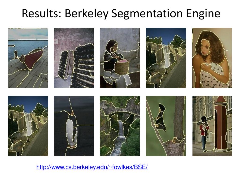
Results: Berkeley Segmentation Engine
53
Normalized cuts: Pro and con
Pros Generic framework, can be used with many different features and affinity formulations Cons High storage requirement and time complexity Bias towards partitioning into equal segments

54
Segments as primitives for recognition?
Multiple segmentations B. Russell et al., “Using Multiple Segmentations to Discover Objects and their Extent in Image Collections,” CVPR 2006

55
Object detection and segmentation
Segmentation energy: D. Ramanan, “Using segmentation to verify object hypotheses,” CVPR 2007

56
Top-down segmentation
E. Borenstein and S. Ullman, “Class-specific, top-down segmentation,” ECCV 2002 A. Levin and Y. Weiss, “Learning to Combine Bottom-Up and Top-Down Segmentation,” ECCV 2006.

57
Top-down segmentation
Normalized cuts Top-down segmentation E. Borenstein and S. Ullman, “Class-specific, top-down segmentation,” ECCV 2002 A. Levin and Y. Weiss, “Learning to Combine Bottom-Up and Top-Down Segmentation,” ECCV 2006.

Similar presentations


 Texture analysis and synthesis Multiple.>")


