1. Visual Description of Data

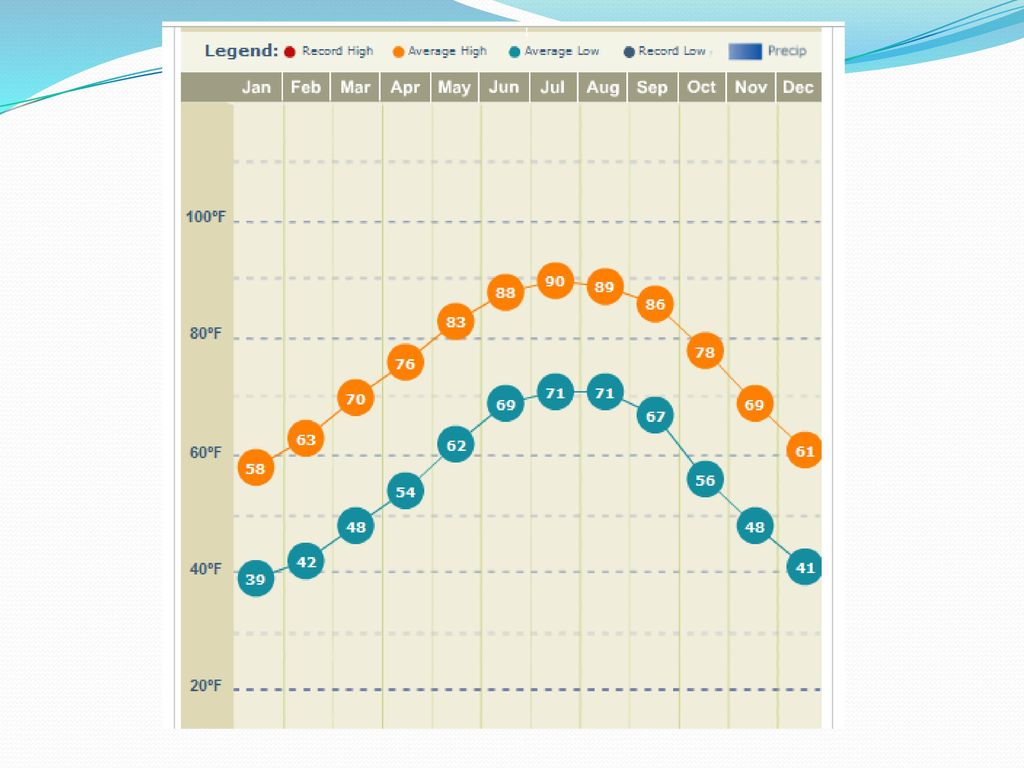
2. Visual description is an art

4. Chapter 2 - Learning Objectives
Convert raw data into a data array.
Construct:
a frequency distribution.
a relative frequency distribution.
a cumulative relative frequency distribution.
Construct a stem-and-leaf diagram.
Construct a histogram.

5. Hospital Cost Problem
The average daily cost to community hospitals for patient stays during 1993 for each of the 50 U.S. states was given in the next table.
a) Arrange these into a data array.
b) Construct a frequency distribution, a relative frequency distribution and a cumulative relative frequency distribution.
c) Construct a stem-and-leaf display.
d) Construct a histogram.

6. The Data
AL $775 HI 823 MA 1,036 NM 1,046 SD 506 AK 1,136 ID 659 MI 902 NY 784 TN 859 AZ 1,091 IL 917 MN 652 NC 763 TX 1,010 AR 678 IN 898 MS 555 ND 507 UT 1,081 CA 1,221 IA 612 MO 863 OH 940 VT 676 CO 961 KS 666 MT 482 OK 797 VA 830 CT 1,058 KY 703 NE 626 OR 1,052 WA 1,143 DE 1,024 LA 875 NV 900 PA 861 WV 701 FL 960 ME 738 NH 976 RI 885 WI 744 GA 775 MD 889 NJ 829 SC 838 WY 537

7. Data Array
CA 1,221 TX 1,010 RI 885 NY 784 KS 666 WA 1,143 NH 976 LA 875 AL 775 ID 659 AK 1,136 CO 961 MO 863 GA 775 MN 652 AZ 1,091 FL 960 PA 861 NC 763 NE 626 UT 1,081 CH 940 TN 859 WI 744 IA 612 CT 1,058 IL 917 SC 838 ME 738 MS 555 OR 1,052 MI 902 VA 830 KY 703 WY 537 NM 1,046 NV 900 NJ 829 WV 701 ND 507 MA 1,036 IN 898 HI 823 AR 678 SD 506 DE 1,024 MD 889 OK 797 VT 676 MT 482

8. The Stem-and-Leaf Display
Stem-and-Leaf Display N = 50 Leaf Unit: , , 81, 58, 52, 46, 36, 24, , 61, 60, 40, 17, 02, 00 (11) 8 98, 89, 85, 75, 63, 61, 59, 38, 30, 29, , 84, 75, 75, 63, 44, 38, 03, , 76, 66, 59, 52, 26, , 37, 07, Range: $482 - $1,221

9. Constructing the Frequency Distribution
Step 1. Number of classes
The range is: $1,221 – $482 = $739
$739/7 ­ $106 and $739/8 ­ $92
Step 2. The class interval
So, if we use 8 classes, we can make each class $100 wide.

10. Constructing the Frequency Distribution
Step 3. The lower class limit
If we start at $450, we can cover the range in 8 classes, each class $100 in width.
The first class : $450 up to $550
Step 4. Setting class limits
$450 up to $550 $850 up to $950
$550 up to $650 $950 up to $1,050
$650 up to $ $1,050 up to $1,150
$750 up to $ $1,150 up to $1,250

11. Frequency Distribution
Average daily cost Number Mark $450 – under $550 4 $500 $550 – under $650 3 $600 $650 – under $750 9 $700 $750 – under $850 9 $800 $850 – under $ $900 $950 – under $1,050 7 $1,000 $1,050 – under $1,150 6 $1,100 $1,150 – under $1,250 1 $1,200 Interval width: $100
We can get this table by using the histogram function in Excel

12. Cumulative Frequency Distribution
Average daily cost Number Cum. Freq. $450 – under $ $550 – under $ $650 – under $ $750 – under $ $850 – under $ $950 – under $1, $1,050 – under $1, $1,150 – under $1,

13. Converting to a Relative Frequency Distribution
1. Retain the same classes defined in the frequency distribution. 2. Sum the total number of observations across all classes of the frequency distribution. 3. Divide the frequency for each class by the total number of observations, forming the percentage of data values in each class.

14. The Relative Frequency Distribution
Average daily cost Number Rel. Freq. $450 – under $ /50 = .08 $550 – under $ /50 = .06 $650 – under $ /50 = .18 $750 – under $ /50 = .18 $850 – under $ /50 = .22 $950 – under $1, /50 = .14 $1,050 – under $1, /50 = .12 $1,150 – under $1, /50 = .02

15. Forming a Cumulative Relative Frequency Distribution
1. List the number of observations in the lowest class. 2. Add the frequency of the lowest class to the frequency of the second class. Record that cumulative sum for the second class. 3. Continue to add the prior cumulative sum to the frequency for that class, so that the cumulative sum for the final class is the total number of observations in the data set.

16. Forming a Cumulative Relative Frequency Distribution
4. Divide the accumulated frequencies for each class by the total number of observations -- giving you the percent of all observations that occurred up to and including that class.
An Alternative: Accrue the relative frequencies for each class instead of the raw frequencies. Then you don’t have to divide by the total to get percentages.

17. The Cumulative Relative Frequency Distribution
Average daily cost Cum.Freq. Cum.Rel.Freq. $450 – under $ /50 = .02 $550 – under $ /50 = .14 $650 – under $ /50 = .32 $750 – under $ /50 = .50 $850 – under $ /50 = .72 $950 – under $1, /50 = .86 $1,050 – under $1, /50 = .98 $1,150 – under $1, /50 = 1.00

18. The Histogram
A histogram is not a bar graph. The x-axis is a qualitative variable.
What is the interval for each class? What are the limits?
How many states are in the group >550 but <=650

19. The Stem-and-Leaf Display
Stem-and-Leaf Display N = 50 Leaf Unit: , , 81, 58, 52, 46, 36, 24, , 61, 60, 40, 17, 02, 00 (11) 8 98, 89, 85, 75, 63, 61, 59, 38, 30, 29, , 84, 75, 75, 63, 44, 38, 03, , 76, 66, 59, 52, 26, , 37, 07, Range: $482 - $1,221
Note similarity and differences with histogram.

20. Summary
Frequency distributions
Stem and leaf plot
Histogram