1. Data Mining: How to make islands of knowledge emerging out of oceans of data Hugues Bersini IRIDIA - ULB

2. PLAN u Rapid intro to data warehouse u data mining: u two super techniques of data mining incomprehensible : Understand and predict Lazy for time series prediction Bagfs for classification

3. The Data Miner Steps u Data Warehousing u Data Preparation –Cleaning + Homogeneisation –Transformation - Composition –Reduction –For time series: time adjustment u Data Modelling : What researchers are mainly interested in.

4. Data Warehouse

7. Re-organization of data u Subject oriented u integrated u transversals u with history u non volatile u from production data ---> to decision-based data

10. Data Mining Uunderstand and predict

11. Modelling the data: only if structure and regularities in the data Data mining IS NOT OLAP To understand the data To predict new data WHY ??

12. The main techniques of data-mining u Clustering u Outlier detection u Association analysis u Forecasting u Classification

13. Data Mining: to understand and/or to predict discovering structure in data discovering I/O relationship in data

14. Nothing new under the sun u New methods extending old ones in the domain of non-linear (NN) and symbolic (decision tree) u Exponential explosion of data u Extracting from huge data base More sensitive than ever

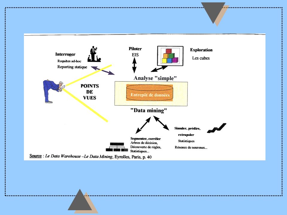
15. CEDITI September 2, 19983 Exploit Exploit Data store Data Store Data volume doubles every 18 months world-wide Problem How to extract relevant knowledge for our decisions from such amounts of data? Solutions Throw it away before using it (most popular) Query it (Query and OLAP tools) Summarize it: extract essence from the bulk according to targeted decision (Data Mining) Decisions

16. Discovering structure in data u When in a space with a metric –Hierarchical clustering –K-Means –NN clustering - Kohonens map u In space without any metric but a cost function: –Grouping Genetic Algorithms....

17. Clustering and outlier

18. Market Basket Analysis: Association analysis Quantity bought

19. Calcul of Improvement

20. Discovering I/O relationship in data ? classificationtime series prediction O = the class I = (x,y) O = x(t+1) I = x(t) t x(t) x y understanding I/O relationship Predicting which O for new I ??

21. Le CV dIRIDIA en data mining u Reconnaissance de défauts vitreux chez Glaverbel u Prediction de fluctuations boursières avec MasterFood et dieteren u Reconnaissance dincidents et prédiction de charge électrique avec Tractebel u Analyse des retards aériens avec Eurocontrôle u Modélisation de Processus Industriel avec Honeywell, FAFER et Siemens u Moteur de recherche Internet convivial avec la Region Wallonne u Classification de pixels pour les images de satelittes

22. Financial prediction Task: predict the future trends of the financial series. Goal: automatic trading system to anticipate the fluctuations of the market.

23. Economic variables Task: predict how many cars will be matriculated next year. Goal: support the marketing campaign of a car dealer.

24. Modeling of industrial plants Task: predict the flow stress of the steel plate as a function of the chemical and physical properties of the material. Rolling steel mill Goal: cope with different types of metals, reduce the production time and improve final quality.

25. Control Task: model the dynamics of the plant on the basis of accessible information. Waste water treatment plant Goal: control the level of water pollutants.

26. Environmental problems Task: predicting the biological state (e.g. density of algae communities) as a function of chemicals. Goal: make automatic the analysis of the state of the river by monitoring chemical concentrations. Algae summer blooming

27. In the medical domain u automatic diagnosis of cancer u detection of respiratory problems u electrocardiogram analysis u help to paraplegic

28. APPLICATION DU DATA MINING DANS LE DOMAINE DU CANCER: Application à l'aide au diagnostic et au pronostic en pathologie tumorale. En collaboration avec le Laboratoire d'Histopathologie (R. Kiss), Faculté de Médecine, U.L.B.

29. patienttumeur chirurgie DIAGNOSTIC (pathologistes) traitement adjuvant bilan clinique critères histologiques: - perte de différenciation - invasion critères cytologiques: - taille des noyaux - mitoses - plages dhyperchromatisme faible, modéré, élevé Amélioration du diagnostic Adéquation du traitement Augmentation de la survie

30. u Exemple: Tumeurs primitives cérébrales (adultes): GLIOMES

31. Objectivation déléments diagnostiques quantification de critères (cytologiques et histologiques) microscopie assistée par ordinateur traitement des données Extraction dinformations diagnostiques et/ou prognostiques fiables et reproductibles

32. 500 à 1000 noyaux par tumeurs. 30 variables tumorales: moyenne déviation standard

33. Application to teledetection

34. Bagfs

35. On internet u The Hyperprisme project u Text Mining u Automatic profiling of users –Key words: positif, negatif,… u Automatic grouping of users on the basis of their profiles u See Web

36. Different approaches Model Data Comprehensible Non comprehensible LocalGlobal Non readable SVM Accuracy of prediction

37. Understanding and Predicting Building Models A model needs data to exist but, once it exists, it can exist without the data. Model Structure Parameters To fit the data Linear, NN, Fuzzy, ID3, Wavelet, Fourier, Polynomes,...

38. From data to prediction RAW DATA PREPROCESSING MODEL LEARNING PREDICTION TRAINING DATA

39. Supervised learning PHENOMENON MODEL input output prediction error Finite amount of noisy observations. No a priori knowledge of the phenomenon. OBSERVATIONS

40. Model learning MODEL GENERATION MODEL VALIDATION PARAMETRIC IDENTIFICATION MODEL SELECTION STRUCTURAL IDENTIFICATION

41. The Practice of Modelling Data + Optimisation Methods Physical Knowledge Engineering Models THE MODEL Rules of Thumb Linguistic Rules Accurate Simple Robust Understandable good for decision

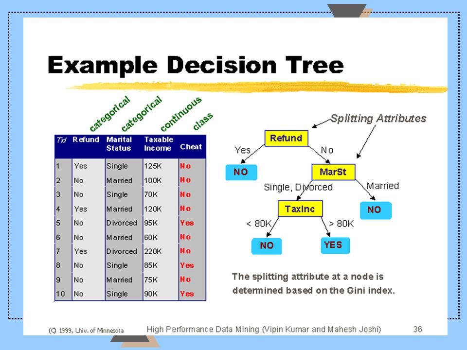
42. Comprehensible models u Decision trees u Qualitative attributes u Force the attributes to be treated separately u classification surfaces parallel to the axes u good for comprehension because they select and separate the variables

43. Decision trees u Very used in practice. One of the favorite data mining methods u Work with noisy data (statistical approaches) can learn logical model out of data expressed by and/or rules u ID3, C4.5 ---> Quinlan u Favoring little trees --> simple models

44. u At every stage the most discriminant attribute u The tree is being constructed top-down adding a new attribute at each level u The choice of the attribute is based on a statistical criteria called : the information gain u Entropie = -p oui log 2 p oui - p non log 2 p non u Entropie = 0 if P oui/non = 1 u Entropie = 1 if P oui/non = 1/2

45. Information gain u S = set of instances, A set of attributes and v set of values of attributes A Gain (S,A) = Entropie(S)- v |S v |/|S|*Entropie(S v ) u the best A is the one that maximises the Gain u The algorithm runs in a recursive way u The same mechanism is reapplied at each level

47. Mais !!!! Is a good client if (x - y)>30000 Salaire mensuel Remboursement demprunt 30000.

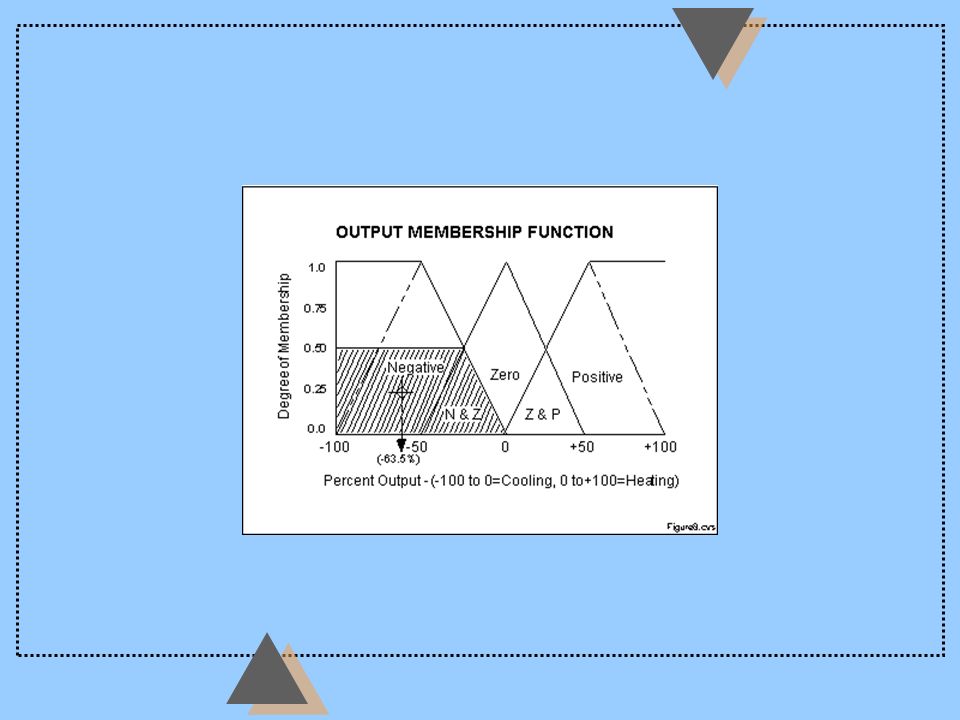
48. Other comprehensible models u Fuzzy logic u Realize an I/O mapping with linguistic rules u If I eat a lot then I take weight a lot

49. Exemple trivial Linéaire, optimal automatique, simple X Y

50. Le flou

54. X Y Si x est très petit alors y est petit Si x est petit alors y est moyen Si x est moyen alors y est moyen lisible ? interfaçable ? adaptatif universel semi-automatique

55. Non comprehensible models u From more to less –linear discriminant –local approaches –fuzzy rules –Support Vector Machine –RBF –global approaches –NN –polynômes, wavelet,… –Support Vector Machine

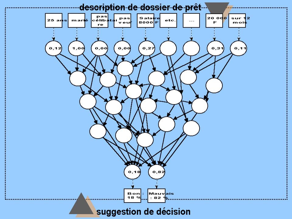
56. Le neuronal

58. précis universel black-box Semi-automatique

59. Nonlinear relationship input output

60. Observations output query

61. Global modeling input output

62. Prediction with global models query

63. Advantages u Exist without data u Information compression t Mainly SVM: mathématiques, pratiques, logique et génériques. u Detect a global structure in the data u Allow to test the sensitivity of the variables u Can easily incorporate prior knowledge

64. Drawbacks u Make assumption of uniformity u Have the bias of their structure u Are hardly adapting u Which one to choose.

65. `Weak classifiers´ ensembles u Classifier capacity reduced in 2 ways : –simplified internal architecture –NOT all the available information u Better generalisation, reducing overfitting u Improving accuracy by decorrelating classifiers errors by increasing the variability in the learning space.

66. Two distinct views of the information u "Vertically", weighting the samples –active learning - not investigated –bagging, boosting, ECOC for multiple classifier systems u "Horizontally", selecting features –feature selection methods –MFS and its extensions. u also : manipulating class label (ECOC) - not investigated yet

67. `Bagging´ : resampling the learning set u Bootstraps aggregating (Leo Breiman) –random and independant perturbation of the learning set. –vital element : instability of the inducer *. t e.g. C4.5, neural network but not kNN ! –increase accuracy by reducing variance * inducer = base learning algorithm : c4.5, kNN,...

68. Learning set resampling : `Arcing´ u Adaptive resampling or reweighting of the learning set (Leo Breiman terminology). Boosting (Freund & Schapire) t sequential reweighting based on the description accuracy. Fe.g. AdaBoost.M1 for multi-class problems. t needs unstability so as bagging t better variability than bagging. t sensible to noisy databases. t better than bagging on non-noisy databases

69. Mutliple Feature Subsets : Stephen D. Bay (1/2) u problem ? –kNN is stable vertically so Bagging doesn't work. horizontally : MFS - combining random selections of features with or without replacement. u question ? –what about other inducers such C4.5 ??

70. u Hypo : kNN uses its horizontal instability. u Two parameters : –K=n/N, proportion of features in subsets. –R, number of subsets to combine. MFS is better than single kNN with FSS and BSS, feature selections techniques. MFS is more stable than kNN on added irrelevant features. MFS decreases variance and bias through randomness. Multiple Feature Subsets : Stephen D. Bay (2/2)

71. BAGFS : a multiple classifier system u BAGFS = MFS inside each Bagging. u BAGMFS = MFS & Bagging together. u 3 parameters –B, number of bootstraps –K=n/N, proportion of features in subsets –R, number of feature subsets u decision rule : majority vote

72. BAGFS architecture around C4.5 not useful

73. Material u 15 UCI continuous databases u 10-fold cross validations u C4.5 Rel 8 with CF=0.25, MINOBJ=2, pruning u no normalisation, no other pre-treatment on data. u majority vote

74. Experiments u Testing parametrization –optimizing K between 0.1 and 1 by means of a nested 10-fold cross-validation –R= 7, B= 7 for two-level method : Bagfs 7x7 –set of 50 classifiers otherwize : Bag 50, BagMfs 50, MFS 50, Boosting 50

75. Experimental Results McNemar test of significance (95%) : Bagfs performs never signif. worse and even sign. better on at least 4 databases (see red databases).

76. u How adjusting the parameters B, K, R –internal cross validation ? –dimensionality and variability measures hypothesis u Interest of a second level ? –About irrelevant and (un)informative features ? –Does bagging + feature selections work better ? –How proving the interest of MFS randomness ? u How using bootstraps complementary ? –Can we ? –What to do ? u How proving horizontal unstability of C4.5 ? u Comparison with 1-level bagging and MFS –Same number of classifiers ? –Advantage of tuning parameters ? BAGFS : discussions

77. BAGFS : next... u More databases –including nominal features –including missing values u Other decision rules : Bayesian approach, ranking,... u Other inducers : LDA, kNN, logistic regr., MLP ?? u Another level : boosting + MFS ?

78. Which best model ?? when they all can perfectly fit the data They all can perfectly fit the data but ! they dont approach the data in the same way. This approach depends on their structure

79. This explains the importance of Cross-validation this value makes the difference Model A vs Model B A Btraining testing

80. Which one to choose u Capital role of crossvalidation. u Hard to run u One possible response

81. u Lazy methods u Coming from fuzzy

82. Model or Examples ?? Build a Model Prediction based on the model Prediction based on the examples

83. A model ? ? ? ?

84. Lazy Methods u Accuracy entails to keep the data and dont use any intermediary model: the best model is the data u Accuracy requires powerful local models with powerful cross-validation methods u Made possible again due to the computer power lazy methods is a new trend which is a revival of an old trend

85. Lazy methods u A lot of expressions for the same thing: –memory-based, instance-based, examples- based,distance-based –nearest-neighbour u lazy for regression, classification and time series prediction u lazy for quantitative and qualitative features

86. Local modeling

87. Prediction with local models query

88. Local modeling procedure The identification of a local model can be summarized in these steps: The thesis focused on the bandwidth selection problem. u Compute the distance between the query and the training samples according to a predefined metric. u Rank the neighbors on the basis of their distance to the query. u Select a subset of the nearest neighbors according to the bandwidth which measures the size of the neighborhood. u Fit a local model (e.g. constant, linear,...).

89. Bias/variance trade-off: overfitting Prediction error too few neighbors overfitting large prediction error

90. Bias/variance trade off: underfitting too many neighbors underfitting large prediction error Prediction error

91. Validation croisée: Press u Fait un leave-one-out sans le faire pour les modèles linéaires u Un gain computationnel énorme u Rend possible une des validations croisées les plus puissantes à un prix computationel infime.

92. Data-driven bandwidth selection (k m ), MSE (k m ) (k M ), MSE (k M ) (k m+1 ), MSE (k m+1 ) MSE (k m )MSE (k m+1 ) MSE (k M ) PREDICTION identification validation identification validation model selection

93. Advantages u No assumption of uniformity u Justified in real life u Adaptive u Simple

94. From local learning to Lazy Learning (LL) u By speeding up the local learning procedure, we can delay the learning procedure to the moment when a prediction in a query point is required (query-by-query learning). u This method is called lazy since the whole learning procedure is deferred until a prediction is required. u Example of non lazy methods (eager) are neural networks where learning is performed in advance, the fitted model is stored and data are discarded.

95. Static benchmarks Datasets: 15 real and 8 artificial datasets from the ML repository. u Methods: Lazy Learning, Local modeling, Feed Forward Neural Networks, Mixtures of Experts, Neuro Fuzzy, Regression Trees (Cubist). u Experimental methodology: 10-fold cross-validation. Results: Mean absolute error, relative error, paired t-test.

96. Observed data Artificial data

97. Experimental results: paired comparison (I) Each method compared with all the others (9*23 =207 comparisons) The lower, the better !!

98. Experimental results: paired comparison (II) Each method compared with all the others (9*23 = 207 comparisons) The larger, the better !!

99. Lazy Learning for dynamic tasks u long horizon forecasting based on the iteration of a LL one-step-ahead predictor. u Nonlinear control – Lazy Learning inverse/forward control. – Lazy Learning self-tuning control. – Lazy Learning optimal control.

100. Dynamic benchmarks u Multi-step-ahead prediction : – Benchmarks: Mackey Glass and 2 Santa Fe time series – Referential methods: recurrent neural networks. u Nonlinear identification and adaptive control : –Benchmarks: Narendra nonlinear plants and bioreactor. –Referential methods: neuro-fuzzy controller, neural controller, linear controller.

101. Santa Fe time series Task: predict the continuation of the series for the next 100 steps.

102. Lazy Learning prediction LL is able to predict the abrupt change around t =1060 !

103. Awards in international competitions u Data analysis competition: awarded as a runner- up among 21 participants at the 1999 CoIL International Competition on Protecting rivers and streams by monitoring chemical concentrations and algae communities. u Time series competition: ranked second among 17 participants to the International Competition on Time Series organized by the International Workshop on Advanced Black-box techniques for nonlinear modeling in Leuven, Belgium

104. Pragmatic conclusions u Comprehension --> decision tree, fuzzy logic u Precision: t global model t lazy methods u You need to be determined on why you do models.