1. 6.5.4 Back-Propagation Computation in Fully-Connected MLP

2. Algorithm 6.3 Forward propagation through a typical deep neural network and the computation of the cost function.

3. 6.5.4 Back-Propagation Computation in Fully-Connected MLP Algorithm 6.4 Backward computation for the deep neural network of algorithm 6.3, which uses in addition to the input x a target y.

4. 6.5.5 Symbol-to-Symbol Derivatives Symbols : variables that do not have specific values Symbolic representations : algebraic and graph-based representations Symbol-to-number di ff erentiation Symbol-to-Symbol di ff erentiation

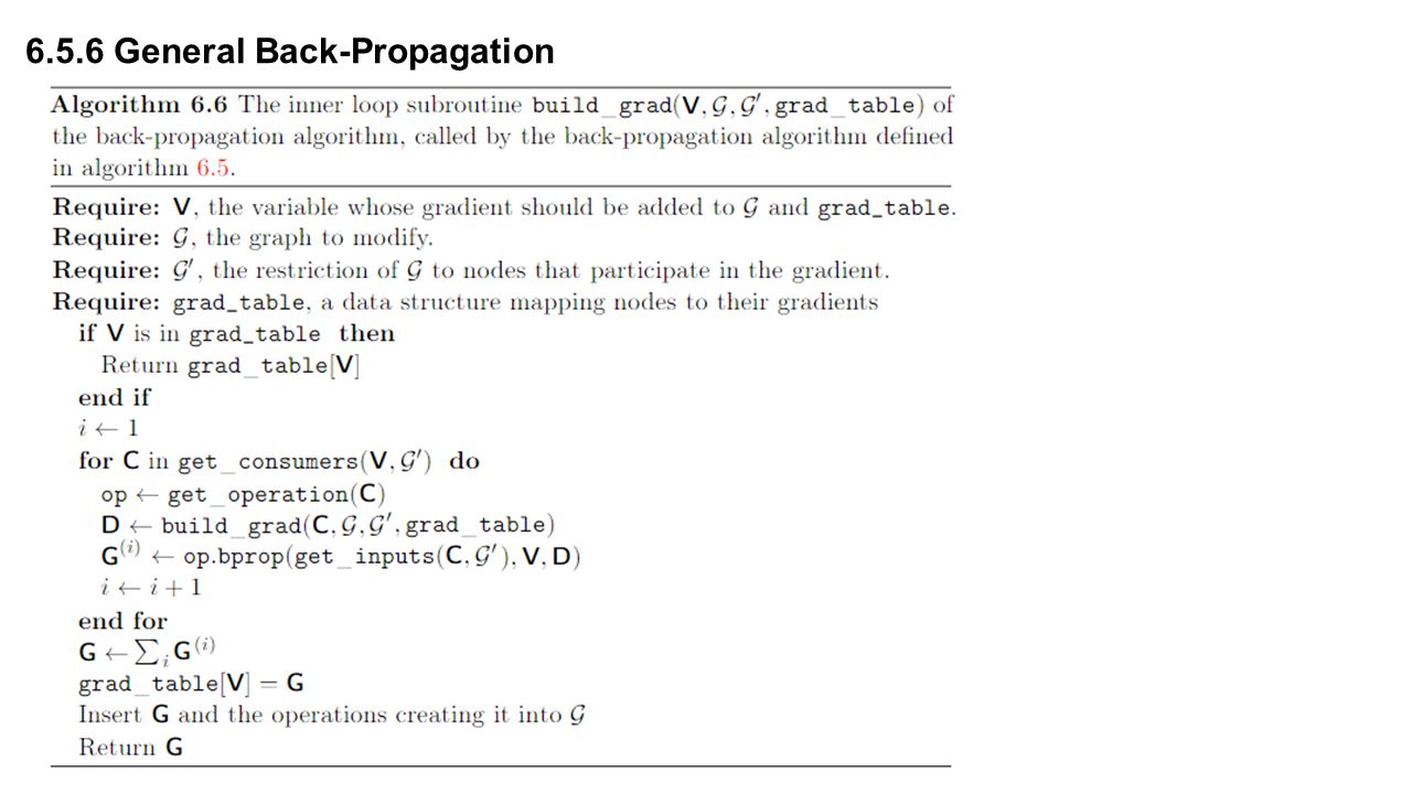
5. 6.5.6 General Back-Propagation

7. dynamic programming : Each node in the graph has a corresponding slot in a table to store the gradient for that node. By filling in these table entries in order, back-propagation avoids repeating many common subexpressions. 6.5.6 General Back-Propagation

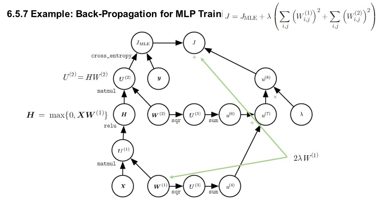
8. 6.5.7 Example: Back-Propagation for MLP Training Single hidden layer matrix to a vector

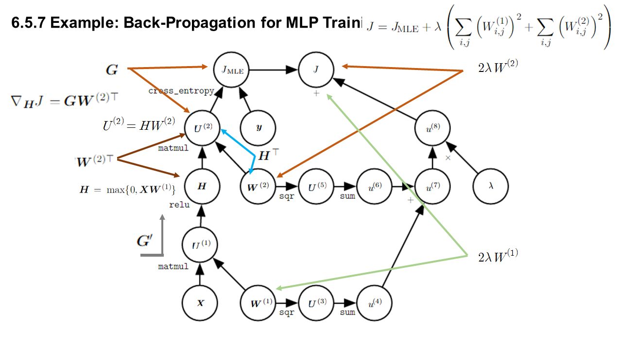
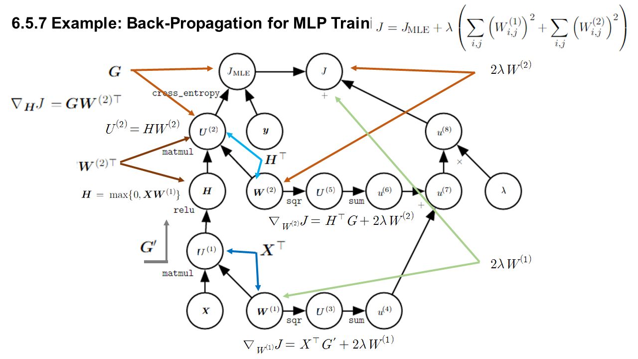
9. 6.5.7 Example: Back-Propagation for MLP Training

18. 6.5.8 Complications Most software implementations need to support operations that can return more than one tensor. Not described how to control the memory consumption of back- propagation. Real-world implementations of back-propagation also need to handle various data types. Some operations have undefined gradients. Various other technicalities make real-world di ff erentiation more complicated.

19. 6.5.9 Di ff erentiation outside the Deep Learning Community When the forward graph has a single output node and each partial derivative can be computed with a constant amount of computation, back-propagation guarantees that the number of computations for the gradient computation is of the same order as the number of computations for the forward computation. In general, finding the optimal sequence of operations to compute the gradient is NP-complete, in the sense that it may require simplifying algebraic expressions into their least expensive form.

20. 6.5.9 Di ff erentiation outside the Deep Learning Community The overall computation is However, it can potentially be reduced by simplifying the computational graph constructed by back-propagation, and this is an NP-complete task. back-propagation can be extended to compute a Jacobian. It is a special case of reverse mode accumulation.

21. 6.5.9 Di ff erentiation outside the Deep Learning Community Forward mode accumulation. When the number of outputs of the graph is larger than the number of inputs. avoids the need to store the values and gradients for the whole graph. trading o ff computational e ffi ciency for memory.

22. 6.5.9 Di ff erentiation outside the Deep Learning Community Forward mode accumulation. For example, if D is a column vector while A has many rows => single output and many inputs cheaper to run the multiplications right-to-left However, if A has fewer rows than D has columns, =>cheaper to run the multiplications left-to-right, corresponding to the forward mode.

23. 6.5.9 Di ff erentiation outside the Deep Learning Community Back-propagation is therefore not the only way or the optimal way of computing the gradient, but it is a very practical method that continues to serve the deeplearning community very well.

24. 6.5.10 Higher-Order Derivatives Some software frameworks support the use of higher-order derivatives. Theano and TensorFlow it is rare to compute a single second derivative of a scalar function we are usually interested in properties of the Hessian matrix. then the Hessian matrix is of size n ×n the typical deep learning approach is to use Krylov methods

25. 6.5.10 Higher-Order Derivatives Krylov methods Krylov methods are a set of iterative techniques for performing various operations like approximately inverting a matrix or finding approximations to its eigenvectors or eigenvalues, without using any operation other than matrix-vector products. Krylov methods on the Hessian, Hessian matrix H and an arbitrary vector. One simply computes