1. Discrete Time Signal Processing Chu-Song Chen （陳祝嵩） song@iis.sinica.edu.tw Institute of Information Science Academia Sinica 中央研究院 資訊科學研究所

2. Textbook Main Textbook Alan V. Oppenheim and Ronald W. Schafer, Discrete-Time Signal Processing, Second Edition, Prentice- Hall, 1999. （全華代理） Reference James. H. McClellan, Ronald W. Schafer, and Mark. A. Yoder, Signal Processing First, Prentice Hall, 2004. （開發代理）

3. Activities Homework – about three times. Tests: twice First test: October 17 Second test: to be announced Term project

4. Teach Assistant 鄭文皇 wisely@cmlab.csie.ntu.edu.tw 通訊與多媒體實驗室 http://www.cmlab.csie.ntu.edu.tw/wisley

5. Contents Discrete-time signals and systems The z-transform Sample of continuous-time signals Transform analysis of linear time invariant systems Structure for discrete-time systems

6. Contents (continue) Filter design techniques The discrete Fourier transform Computation of the discrete Fourier transform Fourier analysis of signals using the discrete Fourier transform

7. Signals Something that conveys information Generally convey information about the state or behavior of a physical system. Signal representation represented mathematically as functions of one or more independent variables.

8. Signal Examples Speech signal: represented as a function over time. -- 1D signal Image signal: represented as a brightness function of two spatial variables. -- 2D signal Ultra sound data or image sequence – 3D signal

9. Signal Types Continuous-time signal defined along a continuum of times and thus are represented by a continuous independent variable. also referred to as analog signal Discrete-time signal defined at discrete times, and thus, the independent variable has discrete values: i.e., a discrete-time signal is represented as a sequence of numbers

10. Signal Types (continue) Digital Signals those for which both time and amplitude are discrete Signal Processing System: map an input signal to an output signal Continuous-time systems Systems for which both input and output are continuous-time signals Discrete-time system Both input and output are discrete-time signals Digital system Both input and output are digital signals

11. Example of Discrete-time Signal Discrete-time signal Discrete-time Signal where n is an integer

12. Generation of Discrete-time Signal In practice, such sequences can often arise from periodic sampling of an analog signal.

13. Signal Operations Multiplication and addition The product and sum of two sequences x[n] and y[n] are defined as the sample-by-sample product and sum, respectively. Multiplication by a number a is defined as multiplication of each sample value by a. Shift operation: y[n] is a delayed or shifted version of x[n] where n 0 is an integer.

14. A Particular Signal Unit sample sequence Unit impulse function, Dirac delta function, impulse

15. Signal Representation An arbitrary sequence can be represented as a sum of scaled, delayed impulses.

16. Some Signal Examples Unit step sequence

17. Some Signal Examples (cont.) Real exponential sequence y[n] can be represented as

18. Some Signal Examples (cont.) Sinusoidal sequence

19. Complex Exponential Sequence Consider an exponential sequence x[n] = A  n, where  is a complex number having real and imaginary parts The sequence oscillates with an exponentialy growing envelope if |  |>1, or with an exponentially decaying envelope if |  |<1

20. Complex Exponential Sequence (cont.) If  =1, the resulted sequence is referred to as a complex exponential sequence and has the form The real and imaginary parts of vary sinusoidally with n. w 0 is called the frequency of the complex exponential and  is called the phase.

21. Discrete and Continuous-time Complex Exponential: Differences We only need to consider frequencies in an interval of length 2 , such as -  <w 0 , or 0  w 0 <2 . Since This property holds also for discrete sinusodial signals: ( r is an integer) This property does not hold for continuous- time complex exponential signals.

22. Another Difference In a continuous-time signal, both complex exponentials and sinusoids are periodic: the period is equal to 2  divided by the frequency. In the discrete-time case, a periodic sequence shall satisfy x[n] = x[n+N], for all n. So, if a discrete-time complex exponential is periodical, then w 0 N = 2  k shall be hold.

23. Example Consider a signal x 1 [n] = cos(  n/4), the signal has a period of N = 8. Let x 2 [n] = cos(3  n/8), which has a higher frequency than x 1 [n] but x 2 [n] is not periodic with period 8, but has a period of N = 16. Contrary to our intuition from continuous-time sinusoids, increasing the frequency of a discrete-time sinusoid does not necessarily decrease the period of the signal. Denote x 3 [n] = cos(n), there exists no integer N satisfying that x 3 [n+N] = x 3 [n].

24. Example (continue) (a) w 0 = 0 or 2  (b) w 0 =  /8 or 15  /8 (c) w 0 =  /4 or 7  /4 (d) w 0 =  As w 0 increases from zero toward  (parts a- d ) the sequence oscillates more rapidly. As w 0 increases from  toward 2  (parts d-a ), the sequence oscillation become slower.

25. Discrete-time Systems A transformation or operator that maps an input sequence with values x[n] into an output sequence with value y[n]. y[n] = T{x[n]} x[n]x[n] T{  } y[n]y[n]

26. System Examples Ideal Delay y[n] = x[n  n d ], where n d is a fixed positive integer called the delay of the system. Moving Average Memoryless Systems The output y[n] at every value of n depends only on the input x[n], at the same value of n. Eg. y[n] = (x[n]) 2, for each value of n.

27. System Examples (continue) Linear System: If y 1 [n] and y 2 [n] are the responses of a system when x 1 [n] and x 2 [n] are the respective inputs. The system is linear if and only if T{x 1 [n] + x 2 [n]} = T{x 1 [n] }+ T{x 2 [n]} = y 1 [n] + y 2 [n]. T{ax[n] } = aT{x[n]} = ay[n], for arbitrary constant a. So, if x[n] =  k a k x k [n], y[n] =  k a k y k [n] (superposition principle) Accumulator System (is a linear system)

28. System Examples (continue) Nonlinear System. Eg. w[n] = log 10 (|x[n]|) is not linear. Time-invariant System: If y[n] = T{x[n]}, then y[n  n 0 ] = T{x[n  n 0 ]} The accumulator is a time-invariant system. The compressor system (not time-invariant) y[n] = x[Mn ],  < n < .

29. System Examples (continue) Causality A system is causal if, for every choice of n 0, the output sequence value at the index n = n 0 depends only the input sequence values for n  n 0. That is, if x 1 [n] = x 2 [n] for n  n 0, then y 1 [n] = y 2 [n] for n  n 0. Eg. Forward-difference system (non causal) y[n] = x[n+1]  x[n] (The current value of the output depends on a future value of the input) Eg. Background-difference (causal) y[n] = x[n]  x[n  1]

30. System Examples (continue) Stability Bounded input, bounded output (BIBO): If the input is bounded, |x[n]|  B x <  for all n, then the output is also bounded, i.e., there exists a positive value B y s.t. |y[n]|  B y <  for all n. Eg., the system y[n] = (x[n]) 2 is stable. Eg., the accumulated system is unstable, which can be easily verified by setting x[n] = u[n], the unit step signal.

31. Linear Time Invariant Systems A system that is both linear and time invariant is called a linear time invariant (LTI) system. By setting the input x[n] as  [n], the impulse function, the output h[n] of an LTI system is called the impulse response of this system. Time invariant: when the input is  [n-k], the output is h[n-k]. Remember that the x[n] can be represented as a linear combination of delayed impulses

32. Hence Therefore, a LTI system is completely characterized by its impulse response h[n]. Linear Time Invariant Systems (continue)

33. Convolution The above operation is called convolution, and can be written in short by y[n] = x[n]  h[n]. In a LTI system, the input sample at n = k, represented as x[k]  [n-k], is transformed by the system into an output sequence x[k]h[n-k] for  < n < . Linear Time Invariant Systems (continue)

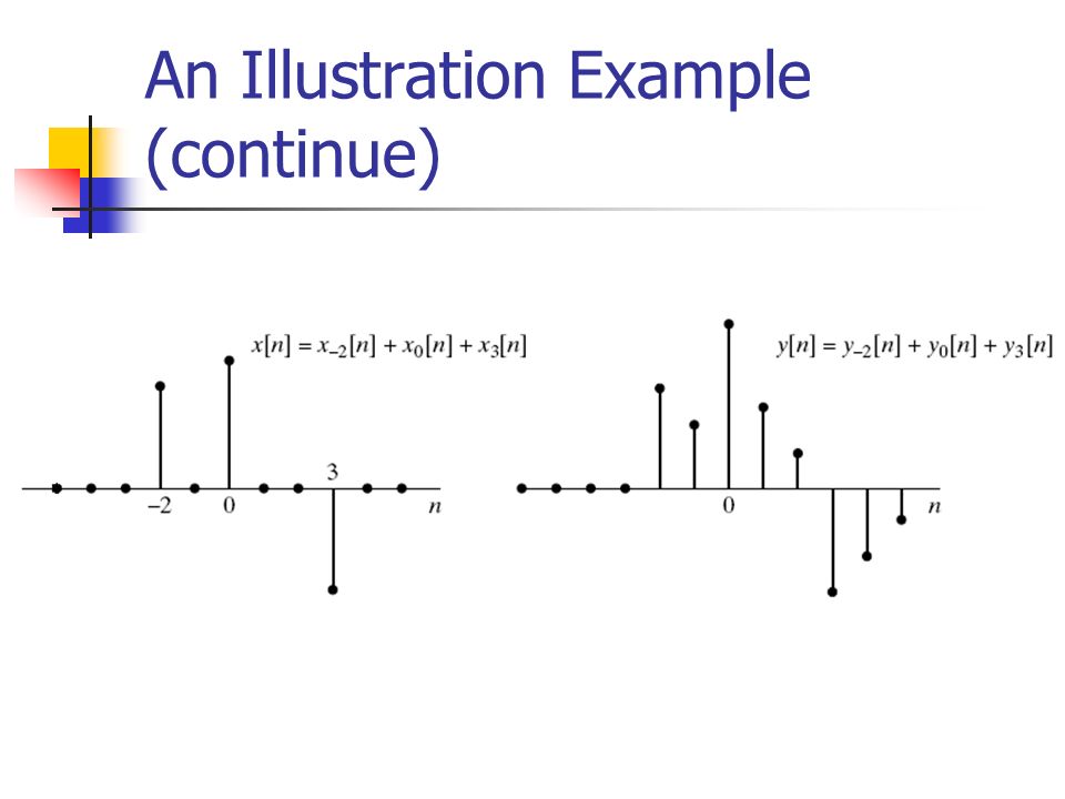
34. An Illustration Example

35. An Illustration Example (continue)

37. Convolution can be realized by Reflecting h[k] about the origin to obtain h[-k]. Shifting the origin of the reflected sequences to k=n. Computing the weighted moving average of x[k] by using the weights given by h[n-k]. Eg., x[n] = 0, 0, 5, 2, 3, 0, 0… h[n] = 0, 0, 1, 4, 3, 0, 0… x[n]  h[n]: Convolution Computation

38. Communitive x[n]  h[n] = h[n]  x[n]. Distributive over addition x[n]  ( h 1 [n] + h 2 [n]) = x[n]  h 1 [n] + x[n]  h 2 [n]. Cascade connection Property of LTI System and Convolution x[n]x[n] h1[n]h1[n]h2[n]h2[n] y[n]y[n]x[n]x[n] h2[n]h2[n]h1[n]h1[n] y[n]y[n] x[n]x[n] h 2 [n]  h2[n] y[n]y[n]

39. Property of LTI System and Convolution (continue) Parallel combination of LTI systems and its equivalent system.

40. Stability: A LTI system is stable if and only if Since when |x[n]|  B x. This is a sufficient condition proof. Property of LTI System and Convolution (continue)

41. Stability: necessary condition to show that if S = , then the system is not BIBO stable, i.e., there exists a bounded input that causes unbounded output. Such a bounded input can be set as ( h*[n] is the complex conjugate of h[n]) In this case, the value of the output at n = 0 is Property of LTI System and Convolution (continue)

42. Causality those systems for which the output depends only on the input samples y[n 0 ] depends only the input sequence values for n  n 0. Follow this property, an LTI system is causal iff h[n ] = 0 for all n < 0. Causal sequence: a sequence that is zero for n <0. A causal sequence could be the impulse response of a causal system. Property of LTI System and Convolution (continue)

43. Ideal delay: h[n ] =  [n-n d ] Moving average Accumulator Forward difference: h[n ] =  [n+1]  [n] Backward difference: h[n ] =  [n]  [n  1] Impulse Responses of Some LTI Systems

44. In the above, moving average, forward difference and backward difference are stable systems, since the impulse response has only a finite number of terms. Such systems are called finite-duration impulse response (FIR) systems. FIR is equivalent to a weighted average of a sliding window. FIR systems will always be stable. The accumulator is unstable since Examples of Stable/Unstable Systems

45. When the impulse response is infinite in duration, the system is referred to as an infinite-duration impulse response (IIR) system. The accumulator is an IIR system. Another example of IIR system: h[n ] = a n u[n] When |a|<1, this system is stable since S = 1 +|a| +|a| 2 +…+ |a| n +…… = 1/(1  |a|) is bounded. When |a|  1, this system is unstable Examples of Stable/Unstable Systems (continue)

46. The ideal delay, accumulator, and backward difference systems are causal. The forward difference system is noncausal. The moving average system is causal requires  M 1  0 and M 2  0. Examples of Causal Systems

47. A LTI system can be realized in different ways by separating it into different subsystems. Equivalent Systems

48. Another example of cascade systems – inverse system. Equivalent Systems (continue)