1. l Basic Definitions: Events, Sample Space, and Probabilities l Basic Rules for Probability l Conditional Probability l Independence of Events l Combinatorial Concepts l The Law of Total Probability and Bayes’ Theorem l Random variables Probability 2

2. l A measure of uncertainty l A measure of the strength of belief in the occurrence of an uncertain event l A measure of the degree of chance or likelihood of occurrence of an uncertain event l Measured by a number between 0 and 1 (or between 0% and 100%)

3. Types of Probability l Objective or Classical Probability based on equally-likely events based on long-run relative frequency of events not based on personal beliefs is the same for all observers (objective) examples: toss a coins, throw a die, pick a card l Subjective Probability –based on personal beliefs, experiences, prejudices, intuition - personal judgment –different for all observers (subjective) –examples: Super Bowl, elections, new product introduction, snowfall

4. Basic Definitions l Set - a collection of elements or objects of interest Empty set (denoted by  ) l a set containing no elements Universal set (denoted by S) l a set containing all possible elements Complement (Not). The complement of A is a set containing all elements of S not in A Intersection (And) – a set containing all elements in both A and B Union (Or) – a set containing all elements in A or B or both

5. Mutually exclusive or disjoint sets - sets having no elements in common, having no intersection, whose intersection is the empty set Collectively exhaustive – If the list of outcomes include all of possible outcomes Partition – a collection of mutually exclusive sets which together include all possible elements, whose union is the universal set Basic Definitions (cont)

6. Partition AB B A A Sets: Diagrams

7. Process that leads to one of several possible outcomes *, e.g.: Coin toss Heads,Tails Throw die 1, 2, 3, 4, 5, 6 Pick a card AH, KH, QH,... Each trial of an experiment has a single observed outcome. The precise outcome of a random experiment is unknown before a trial. * Also called a basic outcome, elementary event, or simple event Experiment

8. l Sample Space or Event Set Set of all possible outcomes (universal set) for a given experiment l E.g.: Throw die S = (1,2,3,4,5,6) l Event Collection of outcomes having a common characteristic l E.g.: Even number A = (2,4,6) Event A occurs if an outcome in the set A occurs l Probability of an event Sum of the probabilities of the outcomes of which it consists l P(A) = P(2) + P(4) + P(6) Events

9. For example: Throw a die Six possible outcomes (1,2,3,4,5,6) If each is equally-likely, the probability of each is 1/6 =.1667 = 16.67% Probability of each equally-likely outcome is 1 over the number of possible outcomes Event A (even number) P(A) = P(2) + P(4) + P(6) = 1/6 + 1/6 + 1/6 = 1/2 for e in A Equally-likely Probabilities

10. Event ‘Ace’ Union of Events ‘Heart’ and ‘Ace’ Event ‘Heart’ The intersection of the events ‘Heart’ and ‘Ace’ comprises the single point circled twice: the ace of hearts Pick a Card: Sample Space

11. l Range of Values l Complements - Probability of not A l Intersection - Probability of both A and B Mutually exclusive events (A and C) : l Range of Values l Complements - Probability of not A l Intersection - Probability of both A and B Mutually exclusive events (A and C) : Basic Rules for Probability (1)

12. Union - Probability of A or B or both Mutually exclusive events: Conditional Probability - Probability of A given B Independent events: Union - Probability of A or B or both Mutually exclusive events: Conditional Probability - Probability of A given B Independent events: Basic Rules for Probability (2)

13. Rules of conditional probability: If events A and D are statistically independent: so Conditional Probability Condition Probability P(A|B) is probability of A given B

14. AT& TIBMTotal Telecommunication401050 Computers203050 Total6040100 Counts AT& TIBMTotal Telecommunication.40.10.50 Computers.20.30.50 Total.60.401.00 Probabilities Probability that a project is undertaken by IBM given it is a telecommunications project: Example (Contingency Table)

15. Conditions for the statistical independence of events A and B: Independence of Events

16. Consider a pair of six-sided dice. There are six possible outcomes from throwing the first die (1,2,3,4,5,6) and six possible outcomes from throwing the second die (1,2,3,4,5,6). Altogether, there are 6*6=36 possible outcomes from throwing the two dice. In general, if there are n events and the event i can happen in N i possible ways, then the number of ways in which the sequence of n events may occur is N 1 N 2... N n. l Pick 5 cards from a deck of 52 - with replacement 52*52*52*52*52=52 5 380,204,032 different possible outcomes l Pick 5 cards from a deck of 52 - without replacement 52*51*50*49*48 = 311,875,200 different possible outcomes Combinatorial Concepts

17. How many ways can you order the 3 letters A, B, and C? There are 3 choices for the first letter, 2 for the second, and 1 for the last, so there are 3*2*1 = 6 possible ways to order the three letters A, B, and C. How many ways are there to order the 6 letters A, B, C, D, E, and F? (6*5*4*3*2*1 = 720) Factorial: For any positive integer n, we define n factorial as: n(n-1)(n-2)...(1). We denote n factorial as n!. The number n! is the number of ways in which n objects can be ordered. By definition 1! = 1. Factorial

18. Permutations are the possible ordered selections of r objects out of a total of n objects. The number of permutations of n objects taken r at a time is denoted nPr. What if we chose only 3 out of the 6 letters A, B, C, D, E, and F? There are 6 ways to choose the first letter, 5 ways to choose the second letter, and 4 ways to choose the third letter (leaving 3 letters unchosen). That makes 6*5*4=120 possible orderings or permutations. Permutations

19. Combinations are the possible selections of r items from a group of n items regardless of the order of selection. The number of combinations is denoted and is read n choose r. An alternative notation is nCr. We define the number of combinations of r out of n elements as: Suppose that when we picked 3 letters out of the 6 letters A, B, C, D, E, and F we chose BCD, or BDC, or CBD, or CDB, or DBC, or DCB. (These are the 6 or 3! permutations or orderings of the 3 letters B, C, and D.) But these are orderings of the same combination of 3 letters. How many combinations of 6 different letters, taking 3 at a time, are there? Combinations

20. In terms of conditional probabilities: More generally (where B i make up a partition): The Law of Total Probability and Bayes’ Theorem

21. Event U: Stock market will go up in the next year Event W: Economy will do well in the next year Example - The Law of Total Probability

22. Bayes’ theorem enables you, knowing just a little more than the probability of A given B, to find the probability of B given A. Based on the definition of conditional probability and the law of total probability. Applying the law of total probability to the denominator Applying the definition of conditional probability throughout Bayes’ Theorem

23. Random Variables A real number is assigned to every outcome or event in an experiment. Outcome is numerical or quantitative  outcome number can be random variable. Outcome is not number  RV so that every outcome corresponding with a unique number. Discrete RV Continuous RV

24. Consider the experiment of tossing two six-sided dice. There are 36 possible outcomes. Let the random variable X represent the sum of the numbers on the two dice: 234567 1,11,21,31,41,51,68 2,12,22,32,42,52,69 3,13,23,33,43,53,610 4,14,24,34,44,54,611 5,15,25,35,45,55,612 6,16,26,36,46,56,6 xP(x) * 21/36 32/36 43/36 54/36 65/36 76/36 85/36 94/36 103/36 112/36 121/36 1 Example

26. A discrete random variable: l has a countable number of possible values l has discrete jumps between successive values l has measurable probability associated with individual values l counts A discrete random variable: l has a countable number of possible values l has discrete jumps between successive values l has measurable probability associated with individual values l counts A continuous random variable: l has an uncountable infinite number of possible values l moves continuously from value to value l has no measurable probability associated with each value l measures (e.g.: height, weight, speed, value, duration, length) A continuous random variable: l has an uncountable infinite number of possible values l moves continuously from value to value l has no measurable probability associated with each value l measures (e.g.: height, weight, speed, value, duration, length) Discrete and Continuous Random Variables

27. The probability distribution of a discrete random variable X sometime is called Probability Mass function, must satisfy the following two conditions. Discrete Probability Distributions - (Probability Mass Function)

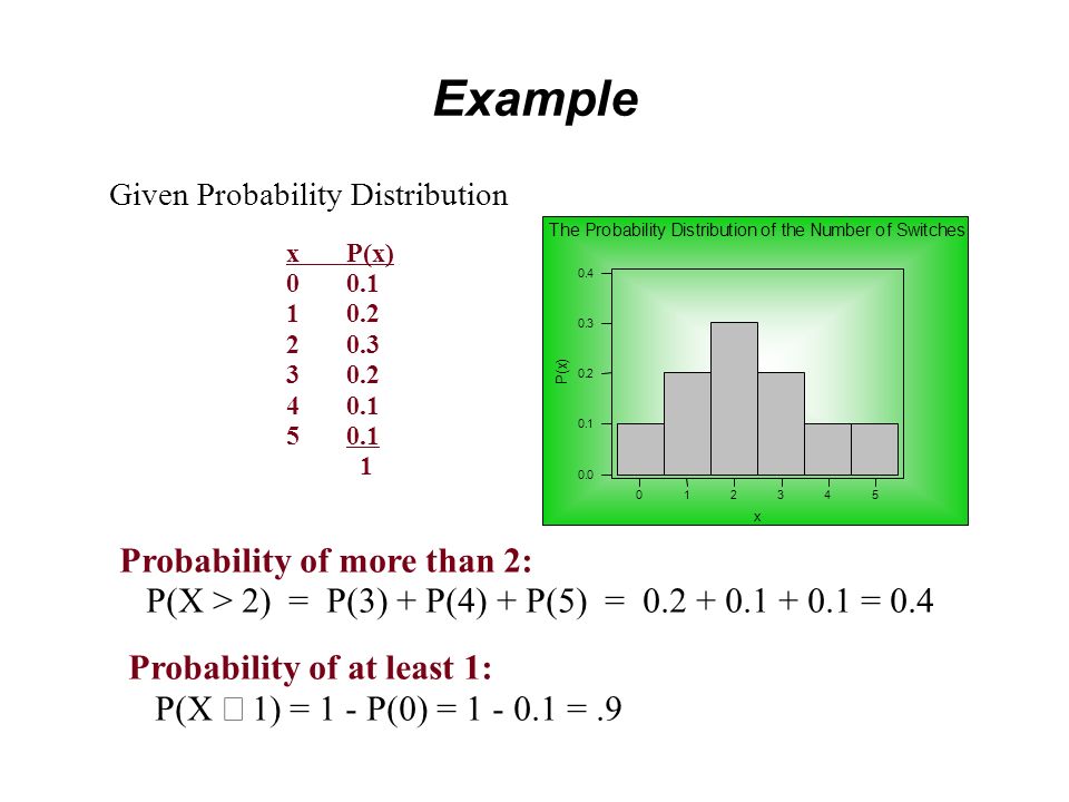
28. The cumulative distribution function, F(x), of a discrete random variable X is: xP(x) F(x) 00.1 0.1 10.2 0.3 20.3 0.6 30.2 0.8 40.1 0.9 50.1 1.0 1 Cumulative Distribution Function (Probability Distribution)

29. xP(x) F(x) 00.1 0.1 10.2 0.3 20.3 0.6 30.2 0.8 40.1 0.9 50.1 1.0 1 The probability that at most three will occur: The Probability That at Most Three Switches Will Occur 543210 0.4 0.3 0.2 0.1 0.0 x P ( x ) Example

30. The mean of a probability distribution is a measure of its centrality or location. The mean is also known as the expected value (or expectation) of a random variable, because it is the value that is expected to occur, on average. The expected value of a discrete random variable X is equal to the sum of each value of the random variable multiplied by its probability. xP(x)xP(x) 00.1 0.0 10.2 0.2 20.3 0.6 30.2 0.6 40.1 0.4 50.1 0.5 1.0 2.3 = E(X)=  Expected Values of Discrete Random Variables

31. Number of items, xP(x)xP(x) g(x)g(x)P(x) 50000.2 10002000400 60000.3 1800 40001200 70000.2 140060001200 80000.2 160080001600 9000 0.1 900100001000 1.0 67005400 Example: Monthly sales of a certain product are believed to follow the probability distribution given below. Suppose the company has a fixed monthly production cost of $8000 and that each item brings $2. Find the expected monthly profit from product sales. The expected value of a function of a discrete random variable X is: Expected Value of a Function of a Discrete Random Variables

32. The variance of a random variable is the expected squared deviation from the mean: The standard deviation of a random variable is the square root of its variance: Variance and Standard Deviation of a Random Variable

33. Bernoulli trials are a sequence of n identical trials satisfying the following conditions: 1. Each trial has two possible outcomes, called success *and failure. The two outcomes are mutually exclusive and exhaustive. 2.The probability of success, denoted by p, remains constant from trial to trial. The probability of failure is denoted by q, where q = 1-p. 3. The n trials are independent. That is, the outcome of any trial does not affect the outcomes of the other trials. A random variable, X, that counts the number of successes in n Bernoulli trials, where p is the probability of success* in any given trial, is said to follow the binomial probability distribution with parameters n (number of trials) and p (probability of success). We call X the binomial random variable. The Binomial Distribution

34. In general: 1. The probability of a given sequence of x successes out of n trials with probability of success p and probability of failure q is equal p x q (n-x) 2. The number of different sequences of n trials that result in exactly x successes is equal to the number of choices of x elements out of a total of n elements. This number is denoted: Binomial Probabilities (Continued)

35. The binomial probability distribution: where : p is the probability of success in a single trial, q = 1-p, n is the number of trials, and x is the number of successes. The Binomial Probability Distribution

36. Mean, Variance, and Standard Deviation of the Binomial Distribution

37. A continuous random variable is a random variable that can take on any value in an interval of numbers. The probabilities associated with a continuous random variable X are determined by the probability density function of the random variable. The function, denoted f(x), has the following properties. 1. f(x)  0 for all x. 2.The probability that X will be between two numbers a and b is equal to the area under f(x) between a and b. 3.The total area under the curve of f(x) is equal to 1.00. The cumulative distribution function of a continuous random variable: F(x) = P(X  x) =Area under f(x) between the smallest possible value of X (often -  ) and the point x. A continuous random variable is a random variable that can take on any value in an interval of numbers. The probabilities associated with a continuous random variable X are determined by the probability density function of the random variable. The function, denoted f(x), has the following properties. 1. f(x)  0 for all x. 2.The probability that X will be between two numbers a and b is equal to the area under f(x) between a and b. 3.The total area under the curve of f(x) is equal to 1.00. The cumulative distribution function of a continuous random variable: F(x) = P(X  x) =Area under f(x) between the smallest possible value of X (often -  ) and the point x. Continuous Random Variables

38. F(x) f(x) x x 0 0 b a F(b) F(a) 1 b a } P(a  X  b) = Area under f(x) between a and b = F(b) - F(a) P(a  X  b)=F(b) - F(a) Probability Density Function and Cumulative Distribution Function

39. As n increases, the binomial distribution approaches a... n = 6n = 14n = 10 6543210 0.3 0.2 0.1 0.0 x P ( x ) Binomial Distribution: n=6, p=.5 109876543210 0.3 0.2 0.1 0.0 x P ( x ) Binomial Distribution: n=10, p=.5 50-5 0.4 0.3 0.2 0.1 0.0 x f ( x ) Normal Distribution:  = 0,  = 1 Normal distribution - Introduction

40. The normal probability density function: 50-5 0.4 0.3 0.2 0.1 0.0 x f ( x ) Normal Distribution:  = 0,  = 1 The Normal Probability Distribution

41. The normal is a family of Bell-shaped and symmetric distributions. because the distribution is symmetric, one-half (.50 or 50%) lies on either side of the mean. Each is characterized by a different pair of mean, , and variance,  . That is: [X~N(   )]. Each is asymptotic to the horizontal axis. The Normal Probability Distribution

42. All of these are normal probability density functions, though each has a different mean and variance. Z~N(0,1) 50-5 0.4 0.3 0.2 0.1 0.0 z f ( z ) Normal Distribution:  =0,  =1 W~N(40,1)X~N(30,25) 454035 0.4 0.3 0.2 0.1 0.0 w f ( w ) Normal Distribution:  =40,  =1 6050403020100 0.2 0.1 0.0 x f ( x ) Normal Distribution:  =30,  =5 Y~N(50,9) 65554535 0.2 0.1 0.0 y f ( y ) Normal Distribution:  =50,  =3 50 Consider: P(39  W  41) P(25  X  35) P(47  Y  53) P(-1  Z  1) The probability in each case is an area under a normal probability density function. Normal Probability Distributions

43. The standard normal random variable, Z, is the normal random variable with mean  = 0 and standard deviation  = 1: Z~N(0,1 2 ). 543210-1-2-3-4-5 0.4 0.3 0.2 0.1 0.0 Z f ( z ) Standard Normal Distribution  =0  =1 { The Standard Normal Distribution

44. z.00.01.02.03.04.05.06.07.08.09 0.00.00000.00400.00800.01200.01600.01990.02390.02790.03190.0359 0.10.03980.04380.04780.05170.05570.05960.06360.06750.07140.0753 0.20.07930.08320.08710.09100.09480.09870.10260.10640.11030.1141 0.30.11790.12170.12550.12930.13310.13680.14060.14430.14800.1517 0.40.15540.15910.16280.16640.17000.17360.17720.18080.18440.1879 0.50.19150.19500.19850.20190.20540.20880.21230.21570.21900.2224 0.60.22570.22910.23240.23570.23890.24220.24540.24860.25170.2549 0.70.25800.26110.26420.26730.27040.27340.27640.27940.28230.2852 0.80.28810.29100.29390.29670.29950.30230.30510.30780.31060.3133 0.90.31590.31860.32120.32380.32640.32890.33150.33400.33650.3389 1.00.34130.34380.34610.34850.35080.35310.35540.35770.35990.3621 1.10.36430.36650.36860.37080.37290.37490.37700.37900.38100.3830 1.20.38490.38690.38880.39070.39250.39440.39620.39800.39970.4015 1.30.40320.40490.40660.40820.40990.41150.41310.41470.41620.4177 1.40.41920.42070.42220.42360.42510.42650.42790.42920.43060.4319 1.50.43320.43450.43570.43700.43820.43940.44060.44180.44290.4441 1.60.44520.44630.44740.44840.44950.45050.45150.45250.45350.4545 1.70.45540.45640.45730.45820.45910.45990.46080.46160.46250.4633 1.80.46410.46490.46560.46640.46710.46780.46860.46930.46990.4706 1.90.47130.47190.47260.47320.47380.47440.47500.47560.47610.4767 2.00.47720.47780.47830.47880.47930.47980.48030.48080.48120.4817 2.10.48210.48260.48300.48340.48380.48420.48460.48500.48540.4857 2.20.48610.48640.48680.48710.48750.48780.48810.48840.48870.4890 2.30.48930.48960.48980.49010.49040.49060.49090.49110.49130.4916 2.40.49180.49200.49220.49250.49270.49290.49310.49320.49340.4936 2.50.49380.49400.49410.49430.49450.49460.49480.49490.49510.4952 2.60.49530.49550.49560.49570.49590.49600.49610.49620.49630.4964 2.70.49650.49660.49670.49680.49690.49700.49710.49720.49730.4974 2.80.49740.49750.49760.49770.49770.49780.49790.49790.49800.4981 2.90.49810.49820.49820.49830.49840.49840.49850.49850.49860.4986 3.00.49870.49870.49870.49880.49880.49890.49890.49890.49900.4990 543210-1-2-3-4-5 0.4 0.3 0.2 0.1 0.0 Z f ( z ) Standard Normal Distribution 1.56 { Standard Normal Probabilities Look in row labeled 1.5 and column labeled.06 to find P(0  z  1.56) =.4406 Finding Probabilities of the Standard Normal Distribution: P(0 ≤ Z ≤ 1.56)

45. To find P(Z<-2.47): Find table area for 2.47 P(0 < Z < 2.47) =.4932 P(Z < -2.47) =.5 - P(0 < Z < 2.47) =.5 -.4932 = 0.0068 543210-1-2-3-4-5 0.4 0.3 0.2 0.1 0.0 Z f ( z ) Standard Normal Distribution Table area for 2.47 P(0 < Z < 2.47) = 0.4932 Area to the left of -2.47 P(Z < -2.47) =.5 - 0.4932 = 0.0068 Finding Probabilities of the Standard Normal Distribution: P(Z < -2.47)

46. To find P(1  Z  2): 1. Find table area for 2.00 F(2) = P(Z  2.00) =.5 +.4772 =.9772 2. Find table area for 1.00 F(1) = P(Z  1.00) =.5 +.3413 =.8413 3. P(1  Z  2.00) = P(Z  2.00) - P(Z  1.00) =.9772 -.8413 =.1359 543210-1-2-3-4-5 0.4 0.3 0.2 0.1 0.0 Z f ( z ) Standard Normal Distribution Area between 1 and 2 P(1  Z  2) =.4772 -.8413 = 0.1359 Finding Probabilities of the Standard Normal Distribution: P(1 ≤ Z ≤ 2)

47. The area within k  of the mean is the same for all normal random variables. So an area under any normal distribution is equivalent to an area under the standard normal. In this example: P(40  X  P(-1  Z  since  and  1009080706050403020100 0.07 0.06 0.05 0.04 0.03 0.02 0.01 0.00 X f ( x ) Normal Distribution:  =50,  =10  = 10 { 543210-1-2-3-4-5 0.4 0.3 0.2 0.1 0.0 Z f ( z ) Standard Normal Distribution 1.0 { Transformation (2) Division by  x ) The transformation of X to Z: The inverse transformation of Z to X: The Transformation of Normal Random Variables (1) Subtraction: (X -  x )

48. Example 4-1 X~N(160,30 2 ) Example 4-2 X~N(127,22 2 ) Using the Normal Transformation

49. The transformation of X to Z: The inverse transformation of Z to X: The transformation of X to Z, where a and b are numbers:: The Transformation of Normal Random Variables