1. Geology 490M 3D Seismic Workshop tom.h.wilson wilson@geo.wvu.edu Department of Geology and Geography West Virginia University Morgantown, WV Demo, Wave Types, and Propagation Paths

7. 127

8. So - to see additional detail in the ground motion - to measure the fractional motion - you need to increase the dynamic range of the recording system. The engineering seismograph we demonstrated in class today is restricted primarily to the shallower applications since events that have traveled great distances will have very small amplitude (less than 1on the scale of ±128. 127

9. Miller et al. 1997 Seismic and GPR methods both record waves that have been reflected from subsurface interfaces. In the one case (GPR) these waves are electromagnetic (and much faster), in the other (Seismic) they are acoustic or mechanical waves.

10. The nice looking seismic sections you’re used to seeing in text books are compiled from field data which is collected in the form of shot records. The disturbances you see in this record consist of different wave types and also of energy traveling along different paths between the source and receiver. handout

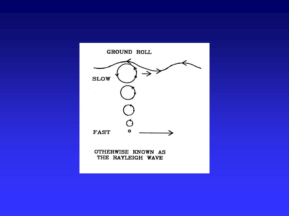
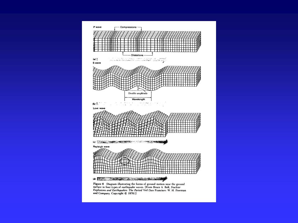
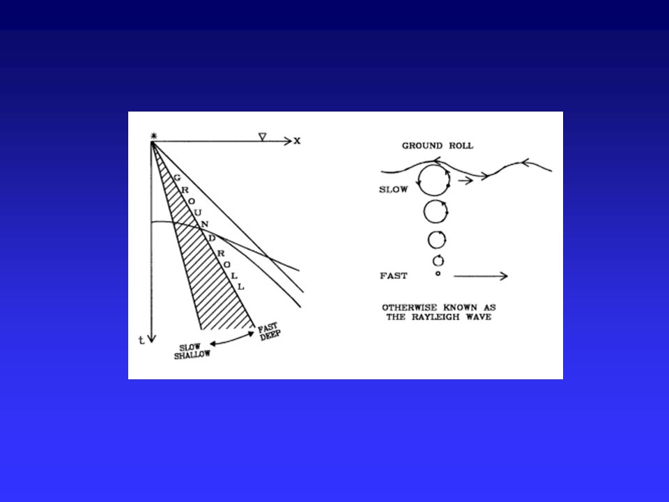
14. In general V R <V L =V S <V P But this is not strictly true. The Love wave is a surface wave and its velocity will be equal to the shear wave velocity in the upper medium. The Love wave like the Rayleigh wave is also a dispersive wave. That means that the deeper extent of the Love wave usually moves more quickly with the shear wave velocity of that deeper medium. V R ~ 0.9V S Shear waves in the beneath the surface layers are generally much faster than those at the surface, so in application, the shear waves that we are concerned with generally have higher velocity than the Love waves.

15. Love waves also tend not to be recorded in a conventional seismic survey where the interest is primarily in the recording of P-waves. The geophones used in such surveys respond to vertical ground motion and so generally do not record the side-to-side vibrations produced by the Love waves. Rayleigh waves produce large vertical displacements and are a significant source of “noise” to those interested in recording the deeper reflection events.

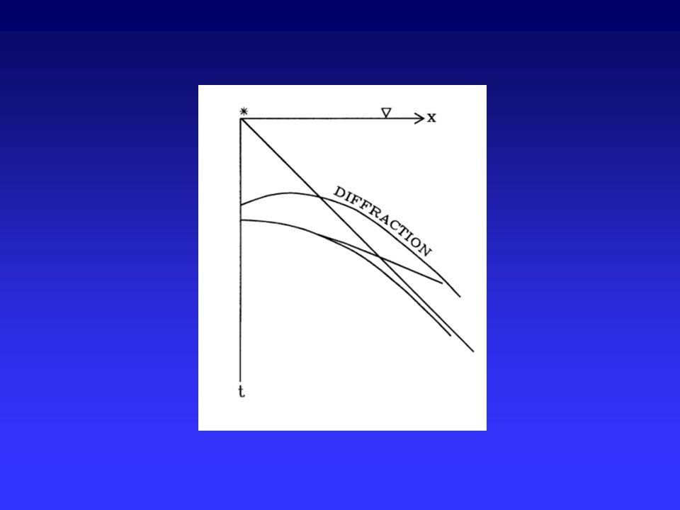
17. How do waves move from one place to another?

19. handout

23. Miller et al. 1995

24. handout

25. Recall Ray-Trace Exercise IV The simulated normal incidence ray-paths have the potential to provide a more accurate visual image of the subsurface. handout

26. Here’s an example of such a data set; the shot locations are obvious aren’t they. We now have a nice geologic looking seismic section. Can you spot the inversion structure? handout

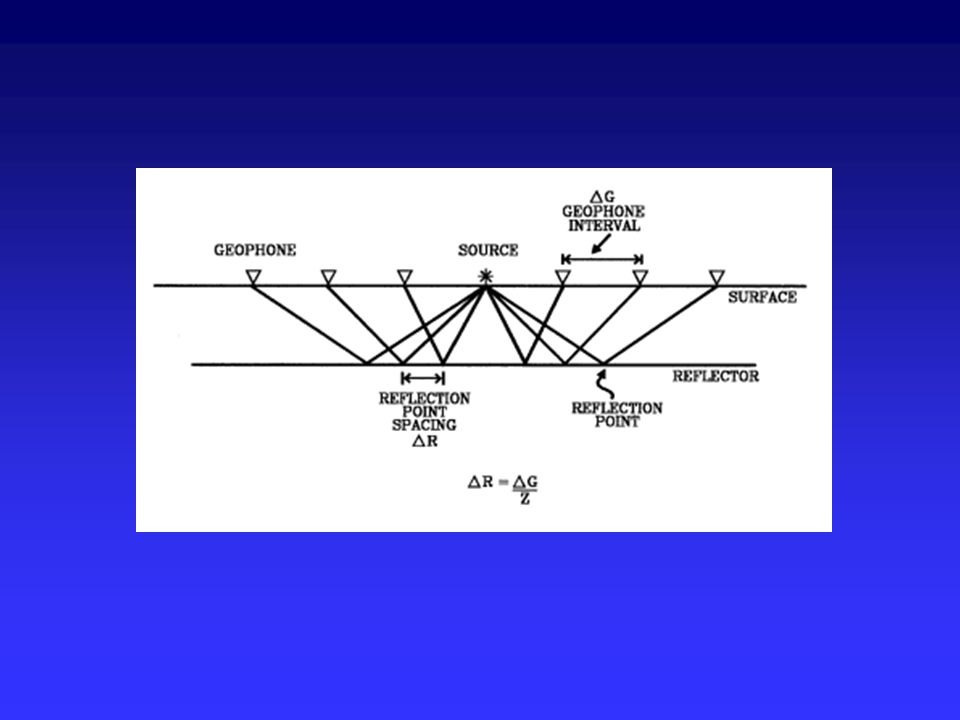
27. Shooting Geometries source receiver layouts used to acquire common midpoint data. Very often these layouts are asymmetrical handout

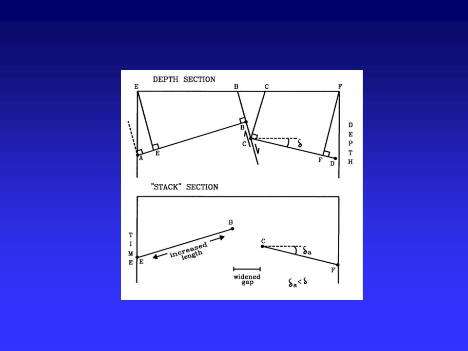
28. The preceding process works well for horizontal or gently dipping strata, but when layers dip, the t-x relationship is asymmetrical and the NMO correction more difficult to make.

29. Common Midpoint Data Reflections share the same midpoint and in this case (horizontal reflector) they also share a common reflection point or depth point handout

31. Three traces in this case (a three fold data set) get summed together to yield one stack trace. The Stack Trace handout

32. What will this CMP reflection event look like in the t-x plot?

33. Even when the layer is dipping, the apex of a reflection hyperbola in the CMP gather (below) is located at x = 0 or at the common midpoint location between all the sources and receivers.

34. Thus the seismic data you will see most often will of this type. The individual traces shown in seismic display will appear to have been collected with coincident source and receiver and, in this format, all the ray paths recorded on the receiver are normal incident on reflection surfaces.

35. Why go to all the trouble of collecting duplicate data? handout

36. A fairly noisy shot record from an area in central West Virginia.

37. Stack Data

38. Common midpoint sorting looks easy on paper

39. In reality (in West Virginia) straight roads are hard to find.

40. Along crooked survey lines, the common midpoint gather includes all records whose midpoints fall within a certain radius of some point Bring the traces inside the circle together for stacking.

41. Noisy single-fold data CMP stack traces

42. Normal incident coincident source-receiver records

43. Some inherent difficulties handout

44. The resulting stack trace handout

45. This data format can lead to some very unusual features in a seismic section. Consider, for example, a survey across a syncline. Consider the distribution of normal incidence ray-paths.

46. Consider what happens across the axis of the syncline and the relation of recording points to reflection points. handout

47. The record of reflection travel time to the various points in the subsurface contains dramatic image distortions - instead of a syncline we have an anticline handout

48. If you think this is only a theoretical construct - think again Pity the poor souls that keeping drilling these “anticlines!”

49. Which structure has the greater reserves?

52. How will the reflections from an isolated point reflector appear in the stack (normal incidence) section. Point reflector

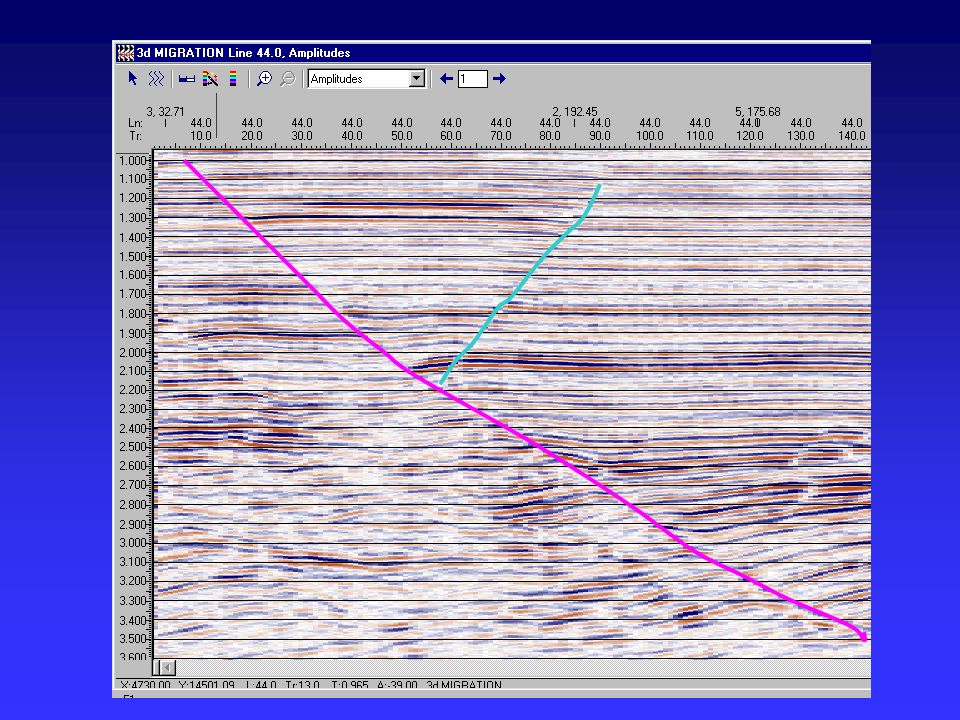
54. Two-D seismic interpretation exercise - You’ll be working with a 3D data base from the Gulf Coast area. So the structures you’ll see will be down-to-basin faults accommodating gravity slide of large portions of the sedimentary section downhill.

56. You have been given 4 seismic lines and a basemap showing their location. By Thursday - please 1) correlate the 1.3 second reflection event on all 4 lines If you want to work ahead … for Next Tuesday we will be doing the following: 1) mark travel time values to the reflector along each line shown on the basemap. Do this often enough to define the major faults and general structure of the 1.3 second horizon 2) contour the travel time data 3) bring your results to class next Tuesday