1. Theoretical distributions: the Normal distribution

2. The Aim By the end of this lecture, the students will be aware of the Normal distribution 2

3. The Goals -Define the terms: probability, conditional probability -Distinguish between the subjective, frequentist and a priori approaches to calculating a probability -Define the addition and multiplication rules of probability -Define the terms: random variable, probability distribution, parameter, statistic, probability density function -Distinguish between a discrete and continuous probability distribution and list the properties of each -List the properties of the Normal and the Standard Normal distributions -Define a Standardized Normal Deviate (SND) 3

4. Normal distribution -Probability -Rules of probabiliyty -Probability distribution -Normal (Gaussian) distibution -Standard normal distribution 4

5. -In previous lectures we showed how to create an empirical frequency distribution of the observed data. -This contrasts with a theoretical probability distribution which is described by a mathematical model. -When our empirical distribution approximates a particular probability distribution, we can use our theoretical knowledge of that distribution to answer questions about the data. -This often requires the evaluation of probabilities. 5

6. Understanding probability -Probability measures uncertainty; it lies at the heart of statistical theory. -A probability measures the chance of a given event occurring. It is a number that takes a value from zero to one. If it is equal to zero, then the event can not occur. If it is equal to one, then the event must occur. -The probability of the complementary event (the event not occurring) is one minus the probability of the event occurring. 6

7. Understanding probability We can calculate a probability using various approaches. Subjective - our personal degree of belief that the event will occur (e.g. that the world will come to an end in the year 2050). Frequentist - the proportion of times the event would occur if we were to repeat the experiment a large number of times (e.g. the number of times we would get a 'head' if we tossed a fair coin 1000 times). A priori - this requires knowledge of the theoretical model, called the probability distribution, which describes the probabilities of all possible outcomes of the 'experiment'. For example, genetic theory allows us to describe the probability distribution for eye colour in a baby born to a blue- eyed woman and brown-eyed man by specifying all possible genotypes of eye colour in the baby and their probabilities. 7

8. The rules of probability We can use the rules of probability to add and multiply probabilities. -The addition rule - if two events, A and B, are mutually exclusive (i.e. each event precludes the other), then the probability that either one or the other occurs is equal to the sum of their probabilities. Prob(A or B) = Prob(A) + Prob(B) For example, if the probabilities that an adult patient in a particular dental practice has -no missing teeth (0.67), -some missing teeth (0.24) or is -edentulous (i.e. has no teeth) (0.09) then the probability that a patient has some teeth is 0.67 + 0.24 = 0.91 8

9. -The multiplication rule - if two events, A and B, are independent (i.e. the occurrence of one event is not contingent on the other), then the probability that both events occur is equal to the product of the probability of each: Prob(A and B) = Prob(A) x Prob(B) For example, if two unrelated patients are waiting in the dentist's surgery, the probability that both of them have no missing teeth is 0.67 X 0.67 = 0.45 9 The rules of probability

10. Probability distributions: the theory -A random variable is a quantity that can take any one of a set of mutually exclusive values with a given probability. -A probability distribution shows the probabilities of all possible values of the random variable. -It is a theoretical distribution that is expressed mathematically, and has a mean and variance that are analogous to those of an empirical distribution. 10

11. Probability distributions: the theory -Each probability distribution is defined by certain parameters which are summary measures (e.g. mean, variance) characterizing that distribution (i.e. knowledge of them allows the distribution to be fully described). -These parameters are estimated in the sample by relevant statistics. -Depending on whether the random variable is discrete or continuous, the probability distribution can be either discrete or continuous. 11

12. Discrete (e.g. Binomial and Poisson) -We can drive probabilities corresponding to every possible value of the random variable. -The sum of all such probabilities is one. 12 Probability distributions: the theory

13. Continuous (e.g. Normal, Chi-squared, t and F) -We can only derive the probability of the random variable, x, taking values in certain ranges (because there are infinitely many values of x). -If the horizontal axis represents the values of x, we can draw a curve from the equation of the distribution (the probability density function); it resembles an empirical relative frequency distribution. -The total area under the curve is one; this area represents the probability of all possible events. -The probability that x lies between two limits is equal to the area under the curve between these values (Fig. 7.1). -For convenience, tables have been produced to enable us to evaluate probabilities of interest for commonly used continuous probability distributions. -These are particularly useful in the context of confidence intervals and hypothesis testing. 13 Probability distributions: the theory

14. 14

15. The Normal (Gaussian) distribution One of the most important distributions in statistics is the Normal distribution. Its probability density function (Fig. 7.2) is: –completely described by two parameters, the mean (µ) and the variance (σ 2 ); –bell-shaped (unimodal); –symmetrical about its mean; –shifted to the right if the mean is increased and to the left if the mean is decreased (assuming constant variance); –flattened as the variance is increased but becomes more peaked as the variance is decreased (for a fixed mean). 15

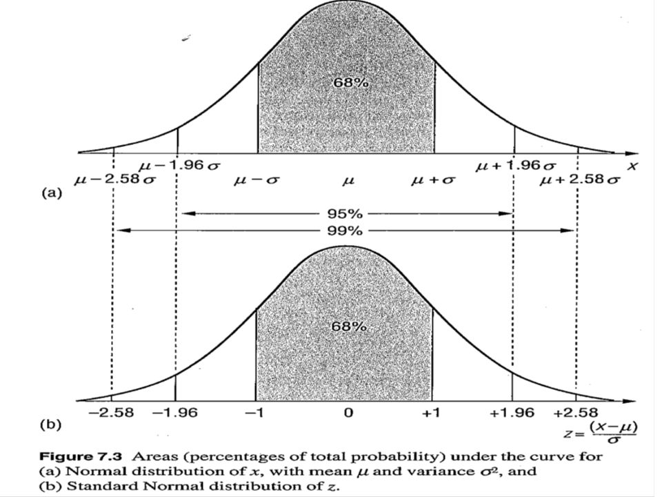
16. The Normal (Gaussian) distribution Additional properties are that: -the mean and median of a Normal distribution are equal; -the probability (Fig. 7.3a) that a Normally distributed random variable, x, with mean, µ, and standard deviation, σ, lies between (µ - σ) and (µ+ σ) is 0.68 (µ - l.96σ) and (µ + 1.96σ) is 0.95 (µ - 2.58σ) and (µ+ 2.58σ) is 0.99 (These intervals may be used to define reference intervals) 16

18. 68-95-99 Rule 68% of the data 95% of the data 99% of the data

20. Copyright © 2007 Pearson Education, Inc Publishing as Pearson Addison-Wesley. Figure 6-12 Converting to a Standard Normal Distribution x –   z =

22. The Normal Distribution X f(X)   Changing μ shifts the distribution left or right. Changing σ increases or decreases the spread.

24. The Normal Distribution: as mathematical function (pdf) Note constants:  =3.14159 e=2.71828 This is a bell shaped curve with different centers and spreads depending on  and 

25. Properties of Normal Distributions A continuous random variable has an infinite number of possible values that can be represented by an interval on the number line. Hours spent studying in a day 06391512182421 The time spent studying can be any number between 0 and 24. The probability distribution of a continuous random variable is called a continuous probability distribution.

26. Properties of Normal Distributions The most important probability distribution in statistics is the normal distribution. A normal distribution is a continuous probability distribution for a random variable, x. The graph of a normal distribution is called the normal curve. Normal curve x

27. The Standard Normal distribution There are infinitely many Normal distributions depending on the values of µ and σ. The Standard Normal distribution (Fig. 7.3b) is a particular Normal distribution for which probabilities have been tabulated. -The Standard Normal distribution has a mean of zero and a variance of one. -If the random variable x has a Normal distribution with mean µ and variance σ 2, then the Standardized Normal Deviate (SND), z = x - µ, is a random variable that has a Standard Normal distribution. 27

29. The Standard Normal Distribution (Z ) All normal distributions can be converted into the standard normal curve by subtracting the mean and dividing by the standard deviation: Somebody calculated all the integrals for the standard normal and put them in a table! So we never have to integrate! Even better, computers now do all the integration.

30. Comparing X and Z units Z 100 2.00 200X (  = 100,  = 50) (  = 0,  = 1)

31. 33 1 22 11 023 z The Standard Normal Distribution The standard normal distribution is a normal distribution with a mean of 0 and a standard deviation of 1. Any value can be transformed into a z - score by using the formula The horizontal scale corresponds to z - scores.

32. The Standard Normal Distribution If each data value of a normally distributed random variable x is transformed into a z - score, the result will be the standard normal distribution. After the formula is used to transform an x - value into a z - score, the Standard Normal Table in Appendix B is used to find the cumulative area under the curve. The area that falls in the interval under the nonstandard normal curve (the x - values) is the same as the area under the standard normal curve (within the corresponding z - boundaries). 33 1 22 11 023 z

33. The Standard Normal Table Properties of the Standard Normal Distribution 1.The cumulative area is close to 0 for z - scores close to z =  3.49. 2.The cumulative area increases as the z - scores increase. 3.The cumulative area for z = 0 is 0.5000. 4.The cumulative area is close to 1 for z - scores close to z = 3.49 z =  3.49 Area is close to 0. z = 0 Area is 0.5000. z = 3.49 Area is close to 1. z 33 1 22 11 023

34. The Standard Normal Table Example : Find the cumulative area that corresponds to a z - score of 2.71. z.00.01.02.03.04.05.06.07.08.09 0.0.5000.5040.5080.5120.5160.5199.5239.5279.5319.5359 0.1.5398.5438.5478.5517.5557.5596.5636.5675.5714.5753 0.2.5793.5832.5871.5910.5948.5987.6026.6064.6103.6141 2.6.9953.9955.9956.9957.9959.9960.9961.9962.9963.9964 2.7.9965.9966.9967.9968.9969.9970.9971.9972.9973.9974 2.8.9974.9975.9976.9977.9978.9979.9980.9981 Find the area by finding 2.7 in the left hand column, and then moving across the row to the column under 0.01. The area to the left of z = 2.71 is 0.9966. Appendix B: Standard Normal Table

35. The Standard Normal Table Example : Find the cumulative area that corresponds to a z - score of  0.25. z.09.08.07.06.05.04.03.02.01.00  3.4.0002.0003  3.3.0003.0004.0005 Find the area by finding  0.2 in the left hand column, and then moving across the row to the column under 0.05. The area to the left of z =  0.25 is 0.4013  0.3.3483.3520.3557.3594.3632.3669.3707.3745.3783.3821  0.2.3859.3897.3936.3974.4013.4052.4090.4129.4168.4207  0.1.4247.4286.4325.4364.4404.4443.4483.4522.4562.4602  0.0.4641.4681.4724.4761.4801.4840.4880.4920.4960.5000 Appendix B: Standard Normal Table

36. The Standard Normal Table What is the area to the left of Z=1.51 in a standard normal curve? Z=1.51 Area is 93.45%

37. Examples

38. Adult IQ scores are normally distributed with  = 100 and  = 15. Estimate the probability that a randomly chosen adult has an IQ between 70 and 115. Solution: Draw the curve. Ex. 3: Estimating a Probability for a Normal Curve

39. Adult IQ scores are normally distributed with  = 100 and  = 15. Estimate the probability that a randomly chosen adult has an IQ between 70 and 115. Solution: Draw the curve. 10085130 115 70 Using the Empirical Rule, the area under the normal curve between these two values is: Area =.135 +.34 +.34 =.815 So the probability the adult has an IQ between 70 and 115 is about.815 Ex. 3: Estimating a Probability for a Normal Curve

40. Guidelines for Finding Areas Example : Find the area under the standard normal curve to the left of z =  2.33. From the Standard Normal Table, the area is equal to 0.0099. Always draw the curve!  2.33 0 z

41. Guidelines for Finding Areas Example : Find the area under the standard normal curve to the right of z = 0.94. From the Standard Normal Table, the area is equal to 0.1736. Always draw the curve! 0.8264 1  0.8264 = 0.1736 0.940 z

42. Guidelines for Finding Areas Example : Find the area under the standard normal curve between z =  1.98 and z = 1.07. From the Standard Normal Table, the area is equal to 0.8338. Always draw the curve! 0.8577  0.0239 = 0.8338 0.8577 0.0239 1.070 z  1.98

43. Probability and Normal Distributions If a random variable, x, is normally distributed, you can find the probability that x will fall in a given interval by calculating the area under the normal curve for that interval. P(x < 15) μ = 10 σ = 5 15μ =10 x

44. Example : The average on a statistics test was 78 with a standard deviation of 8. If the test scores are normally distributed, find the probability that a student receives a test score less than 90. Probability and Normal Distributions P(x < 90) = P(z < 1.5) = 0.9332 The probability that a student receives a test score less than 90 is 0.9332. μ =0 z ? 1.5 90μ =78 P(x < 90) μ = 78 σ = 8 x

45. Example : The average on a statistics test was 78 with a standard deviation of 8. If the test scores are normally distributed, find the probability that a student receives a test score greater than than 85. Probability and Normal Distributions P(x > 85) = P(z > 0.88) = 1  P(z < 0.88) = 1  0.8106 = 0.1894 The probability that a student receives a test score greater than 85 is 0.1894. μ =0 z ? 0.88 85μ =78 P(x > 85) μ = 78 σ = 8 x

46. Example : The average on a statistics test was 78 with a standard deviation of 8. If the test scores are normally distributed, find the probability that a student receives a test score between 60 and 80. Probability and Normal Distributions P(60 < x < 80) = P(  2.25 < z < 0.25) = P(z < 0.25)  P(z <  2.25) The probability that a student receives a test score between 60 and 80 is 0.5865. μ =0 z ?? 0.25  2.25 = 0.5987  0.0122 = 0.5865 6080μ =78 P(60 < x < 80) μ = 78 σ = 8 x

47. Summary Normal distribution -Probability -Rules of probabiliyty -Probability distribution -Normal (Gaussian) distibution -Standard normal distribution 47