Download presentation
Presentation is loading. Please wait.

1
Lecture 1.4. Sampling. Kotelnikov-Nyquist Theorem.

2
Ideal Sampling and Nyquist Theorem Impulse Sampling and Digital Signal Processing Ideal Sampling and Reconstruction Nyquist Rate Aliasing (наложение спектров) Problem Dimensionality Theorem Reconstruction Using Zero Order Hold.
 Problem Dimensionality Theorem Reconstruction Using Zero Order Hold.")
3
Bandlimited Waveforms Definition: A waveform w(t) is limited (Absolutely Bandlimited) to B hertz if W(f) = ℑ [w(t)] = 0 for |f| ≥ B Definition: A waveform w(t) is (Absolutely Time Limited) if w(t) = 0, for |t| ≥ T Theorem: An absolutely bandlimited waveform cannot be absolutely time limited, and vice versa. A physical waveform that is time limited, may not be absolutely bandlimited, but it may be bandlimited for all practical purposes in the sense that the amplitude spectrum has a negligible level above a certain frequency. |W(f)| f 0 Bandlimited B -B-B
![Bandlimited Waveforms Definition: A waveform w(t) is limited (Absolutely Bandlimited) to B hertz if W(f) = ℑ [w(t)] = 0 for |f| ≥ B Definition: A waveform w(t) is (Absolutely Time Limited) if w(t) = 0, for |t| ≥ T Theorem: An absolutely bandlimited waveform cannot be absolutely time limited, and vice versa.](http://images.slideplayer.com/42/11239165/slides/slide_3.jpg "A physical waveform that is time limited, may not be absolutely bandlimited, but it may be bandlimited for all practical purposes in the sense that the amplitude spectrum has a negligible level above a certain frequency. |W(f)| f 0 Bandlimited B -B-B.")
4
Sampling Theorem Sampling Theorem: Any physical waveform may be represented over the interval -∞ < t < ∞ by The f s is a parameter called the Sampling Frequency. Furthermore, if w(t) is bandlimited to B Hertz and f s ≥ 2B, then above expansion becomes the sampling function representation, where a n = w(n/f s ) That is, for f s ≥ 2B, the orthogonal series coefficients are simply the values of the waveform that are obtained when the waveform is sampled with a Sampling Period of T s =1/ f s seconds.
 is bandlimited to B Hertz and f s ≥ 2B, then above expansion becomes the sampling function representation, where a n = w(n/f s ) That is, for f s ≥ 2B, the orthogonal series coefficients are simply the values of the waveform that are obtained when the waveform is sampled with a Sampling Period of T s =1/ f s seconds..")
5
Sampling Theorem The MINIMUM SAMPLING RATE allowed for reconstruction without error is called the NYQUIST FREQUENCY or the Nyquist Rate. Suppose we are interested in reproducing the waveform over a T 0 -sec interval, the minimum number of samples that are needed to reconstruct the waveform is: There are N orthogonal functions in the reconstruction algorithm. We can say that N is the Number of Dimensions needed to reconstruct the T 0 -second approximation of the waveform. The sample values may be saved, for example in the memory of a digital computer, so that the waveform may be reconstructed later, or the values may be transmitted over a communication system for waveform reconstruction at the receiving end.

6
Sampling Theorem

7
Impulse Sampling and Digital Signal Processing The impulse-sampled series is another orthogonal series. It is obtained when the (sin x) / x orthogonal functions of the sampling theorem are replaced by an orthogonal set of delta (impulse) functions. The impulse-sampled series is identical to the impulse-sampled waveform w s (t): both can be obtained by multiplying the unsampled waveform by a unit-weight impulse train, yielding Waveform Impulse sampled waveform
 / x orthogonal functions of the sampling theorem are replaced by an orthogonal set of delta (impulse) functions. The impulse-sampled series is identical to the impulse-sampled waveform w s (t): both can be obtained by multiplying the unsampled waveform by a unit-weight impulse train, yielding Waveform Impulse sampled waveform.")
8
Reconstruction of a Sampled Waveform The sampled signal is converted back to a continuous signal by using a reconstruction system such as a low pass filter. x(nT s ) Same sample values may give different reconstructed signals x 1 (t) and x 2 (t). Why ???
 Same sample values may give different reconstructed signals x 1 (t) and x 2 (t). Why .")
9
Ideal Reconstruction in the Time Domain The sampled signal is converted back to a continuous signal by using a reconstruction system such as a low pass filter having a Sa function impulse response x(nT s ) The impulse response of the ideal low pass reconstruction filter. Ideal low pass reconstruction filter output.

10
Spectrum of a Impulse Sampled Waveform The spectrum for the impulse-sampled waveform w s (t) can be evaluated by substituting the Fourier series of the (periodic) impulse train into above Eq. to get By taking the Fourier transform of both sides of this equation, we get

11
Spectrum of a Impulse Sampled Waveform The spectrum of the impulse sampled signal is the spectrum of the unsampled signal that is repeated every f s Hz, where f s is the sampling frequency (samples/sec). This is quite significant for digital signal processing (DSP). This technique of impulse sampling maybe be used to translate the spectrum of a signal to another frequency band that is centered on some harmonic of the sampling frequency.
. This technique of impulse sampling maybe be used to translate the spectrum of a signal to another frequency band that is centered on some harmonic of the sampling frequency..")
12
Undersampling and Aliasing If f s <2B, The waveform is Undersampled. The spectrum of w s (t) will consist of overlapped, replicated spectra of w(t). The spectral overlap or tail inversion, is called aliasing or spectral folding. The low-pass filtered version of w s (t) will not be exactly w(t). The recovered w(t) will be distorted because of the aliasing. Low Pass Filter for Reconstruction Notice the distortion on the reconstructed signal due to undersampling
 will consist of overlapped, replicated spectra of w(t). The spectral overlap or tail inversion, is called aliasing or spectral folding. The low-pass filtered version of w s (t) will not be exactly w(t). The recovered w(t) will be distorted because of the aliasing. Low Pass Filter for Reconstruction Notice the distortion on the reconstructed signal due to undersampling.")
13
Undersampling and Aliasing Effect of Practical S ampling Effect of Practical S ampling Notice that the spectral components have decreasing magnitude

14
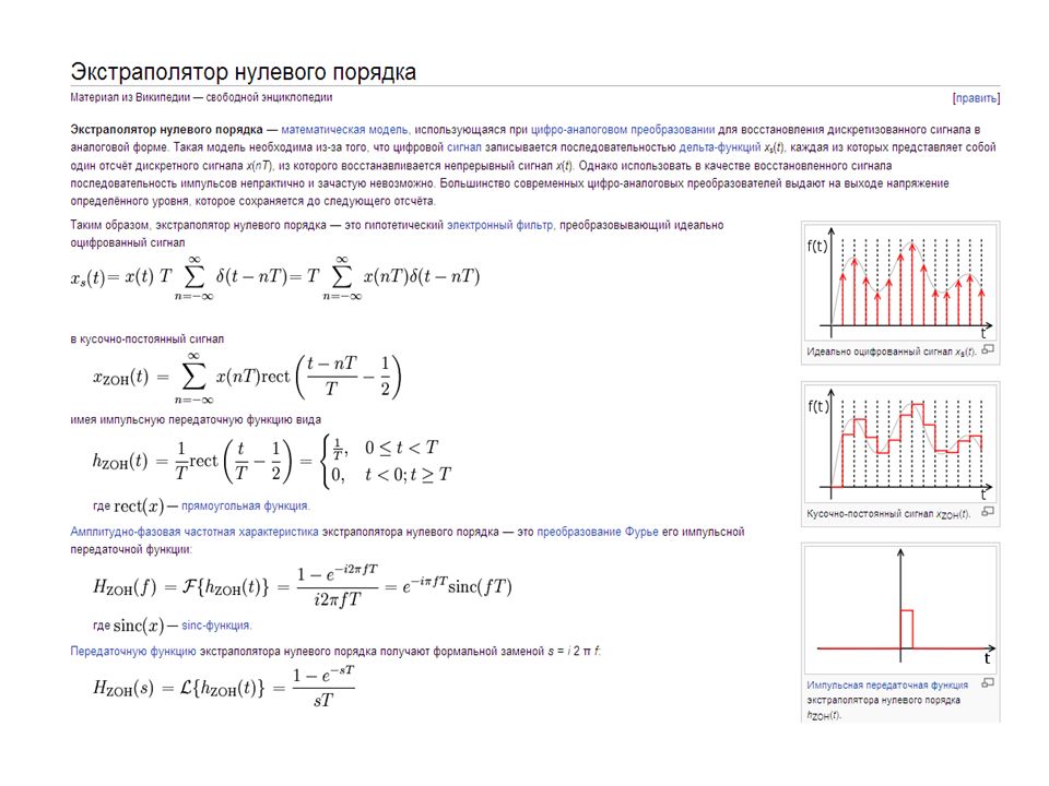
Reconstruction Using a Zero-order Hold Basic System Anti-imaging Filter is used to correct distortions occurring due to non ideal reconstruction

16
Discrete Processing of Continuous-time Signals Basic System Equivalent Continuous Time System

17
END

Similar presentations


,>")


: Sampling theorem, discrete Fourier transform.>")


 is an infinite series of delta functions with a period.>")