1. Spectroscopy – Continuous Opacities I. Introduction: Atomic Absorption Coefficents II. Corrections for Stimulated Emission III. Hydrogen IV. Negative Hydrogen Ion V. Negative Helium Ion VI. Metals VII. Electron Scattering VIII. Others IX. Summary

2. In order to calculate the transer of radiation through a model stellar atmosphere, we need to know the continuous absorption coefficient, . This shapes the continous spectrum → more absorption, less light. It also influences the strength of stellar lines → more continous absorption means a thinner photosphere with few atoms to make spectral lines. Also, before we computer a theoretical spectrum, you need to compute an atmospheric model, and this also depends on .

3. I. The atomic absorption coefficent The total continuous absorption coefficient is the sum of absorption resulting from many physical processes. These are in two categories: bound-free transition: ionization free-free transition: acceleration of a charge when passing another charge bound-bound transitions result in a spectral line and are not included in  but in cool stars line density is so great it affects the continuum

6. B1I V F0 V G2 V

7. I. The atomic absorption coefficent The atomic absorption coefficient, , has units of area per absorber. The wavelength versus frequency question does not arise for  :  =   is not a distribution like I and I, but the power subtracted from I in interval d is  d. This is a distribution and has units of erg/(s cm 2 rad 2 Hz)  d =(c/ 2 )  d

8. II. Corrections for Stimulated Emission Recall that the stimulated emission (negative absorption) reduces the absorption:   = N ℓ B ℓu h – N u B uℓ h = N ℓ ℓ u h (1– N u B uℓ /N ℓ B ℓu ) = N ℓ B ℓu h [1– exp(–h /kT)] B ul B lu NuNu NℓNℓ ℓ

9. T cm K T 1 – exp(h /kT) % decrease 0.240000.9990.08 0.480000.9732.8 0.6120000.90910.0 0.8160000.83419.8 1.0200000.76331.1 T eff (10% reduction) 300002500 Ang 3000 2m2m

10. · · · 0.00 10.20 12.08 12.75 13.60 Lyman n=1 n=2 n=3 n=4 n= ∞ BalmerPachen Brackett  = 13.6(1–1/n 2 ) eV ½ mv 2 = h –hRc/n 2 R = 1.0968×10 5 cm –1 III. Atomic Absorption Coefficient for Hydrogen HH 

11. 2 3647 Balmer 3 8206 Paschen 4 14588 Brackett 5 22790 Pfund At the ionization limit v=0, =Rc/n 2 ½ mv 2 = h –hRc/n 2 R = 1.0968×10 5 cm –1 n Ang Name 1 912 Lyman Absorption edges:

12. III. Neutral Hydrogen: Bound-Free Original derivation is from Kramers (1923) and modified by Gaunt (1930):  n = 6.16 e6e6 h R n 5 3 gn∕gn∕  n = 6.16 e6e6 h3c3h3c3 R gn∕gn∕ 3 n5n5 = 00 gn∕gn∕  n5n5 a 0 = 1.044×10 –26 for in angstroms e = electron charge = 4.803×10 –10 esu gn∕gn∕ = Gaunt factor needed to make Kramer´s result in agreement with quantum mechanical results Per neutral H atom

13.  0, 10× –17 cm 2 /H atom Wavelength (Angstroms) n =1 n =2 n =1 n =2 n =3 n =1 n =2 n =3 n = 4 n =1 n =2 n =3 n = 4 n = 5 n =1 n =2 n =3 n = 4 n = 5 n = 6 n =1 n =2 n =3 n = 4 n = 5 n = 6 n = 7 n =1 n =2 n =3 n = 4 n = 5 n = 6 n = 7 ~ 3 /n 5 ~ 3

14. The sum of absorbers in each level times  n is what is needed. Recall: NnNn N = gngn u 0 (T) ( kT ) – exp  g n =2n 2  =I – hRc/n 2 = 13.6(1-1/n 2 ) eV u 0 (T) = 2 III. Neutral Hydrogen: Bound-Free

15. The absorption coefficient in square centimeters per neutral hydrogen atom for all continua starting at n 0  (H bf ) = Σ n0n0 ∞ nNnnNn N =  0 Σ n0n0 ∞ 3 n3n3 gn∕gn∕ ( kT ) – exp  =  0 Σ n0n0 ∞ 3 n3n3 gn∕gn∕ 10 –  III. Neutral Hydrogen: Bound-Free  = 5040/T,  in electron volts

16. Unsöld showed that the small contributions due to terms higher than n 0 +2 can be replaced by an integral: Σ n 0 +3 ∞ 1 n3n3 ( kT ) – exp  = ½ ∫ n 0 +3 ∞ ( kT ) – exp  d(1/n 2 )  =I – hRc/n 2 => d  = –Id(1/n 2 ) Σ n 0 +3 ∞ 1 n3n3 ( kT ) – exp  = ½ ∫ 33 I ( kT ) – exp  dd I  3 = I [ 1– 1 (n 0 +3) 2 ] III. Neutral Hydrogen: Bound-Free = kT I [ ( – exp   ) ( kT – exp  ) ] –

17. We can neglect the n dependence on g n ∕ and the final answer is: This is the bound free absorption coefficient for neutral hydrogen  (H bf ) =  0 3 [ Σ n0n0 n 0 +2 gn∕gn∕ n3n3 10 –  + log e 2I2I (10 –  3  – 10 –I  ) ] III. Neutral Hydrogen: Bound-Free

18.  bf (>3647)  bf (<3647) =  bf (n=3) +...  bf (n=2) +  bf (n=3) +... ≈  bf (n=3)  bf (n=2) 8 = 27 exp [ [ –(  3 –  2 )/kT = 0.0037 at 5000 K and 0.033 at 10000 K

19. edge (Ang) T 3000 T 5000 T 10000 T 30000 Lyman  9×10 –19 6×10 –12 9×10 –7 0.002 Balmer36470.000210.003760.0330.14 Paschen82060.030.0890.1770.31 Brackett145880.160.2550.360.45 Pfund227900.300.390.480.54 III. Neutral Hydrogen: Bound-Free  (red side)/  (blue side)

20. III. Neutral Hydrogen: Bound-Free

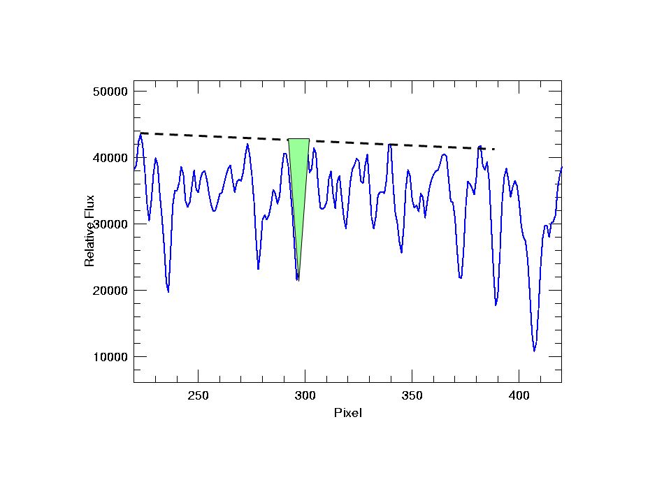
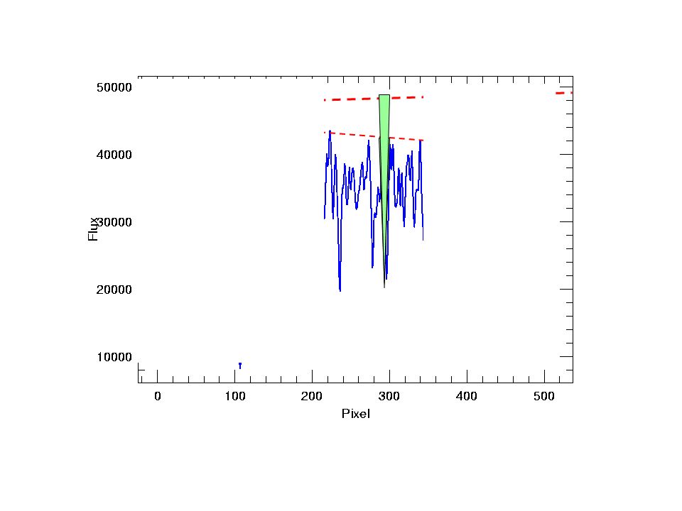
21. III. Optical Depth and Height of Formation Wavelength Flux 91236478602 Recall:  =   dx  ~ 2/3 for Grey atmosphere As  increases,  increases => dx decreases You are looking higher in the atmosphere continuum Across a jump your are seeing very different heights in the atmosphere

22. <3647 A  =2/3 >3647 A  =2/3 z=0 Temperature profile of photosphere 10000 8000 6000 4000 z=0 Temperature z z dx 1 dx 2  (  (>3647) => dx 2 > dx 1

23. B4 V

24. Wavelength (Ang) Amplitude (mmag) Amplitude of rapidly oscillating Ap stars: Different wavelengths probe different heights in atmosphere

25. III. Neutral Hydrogen: Free-Free The free-free absorption of hydrogen is much smaller. When the free electron has a collision with a proton its unbound orbit is altered. The electron absorbs the photon and its energy increases. The strength of this absorption depends on the velocity of the electron

26. III. Neutral Hydrogen: Free-Free proton e–e– Orbit is altered The absorption of the photon is during the interaction

27. III. Neutral Hydrogen: Free-Free Absorption According to Kramers the atomic coefficient is: d  ff = 0.385 h  e 2 R m3m3 1 3 v dv This is the cross section in square cm per H atom for the fraction of the electrons in the velocity interval v to v + dv. To get complete f-f absorption must integrate over v.

28. Using the Maxwell-Boltzmann distribution for v  ff = 0.385 h  e 2 R m3m3 1 3 ( m kT ) 2 3 exp ( mv2mv2 2kT ) – v ( 2  ) 2 1 ∫ 0 ∞ dv ( 2m  kT )  ff = 0.385 h  e 2 R m3m3 3 1 2 1 Quantum mechanical derivation by Gaunt is modified by f-f Gaunt factor g f III. Neutral Hydrogen: Free-Free Absorption

29. The absorption coefficient in square cm per neutral H atom is proportional to the number density of electrons, N e and protons N i :  (H ff ) = fgfNiNefgfNiNe N0N0 Density of neutral H Recall the Saha Equation: ( 2 3 2 5 = NiNi N PePe h3h3 2m2m ) ( kT ) 2u 1 (T) u 0 (T) ( kT ) – exp I P e = N e kT III. Neutral Hydrogen: Free-Free Absorption

30.  (H ff ) = fgffgf 2 3 ( 2  mkT ) h3h3 ( kT ) – exp I  I  (H ff ) =  0 3 g f log e 10 –  I Using: I=hcR R=2  2 me 4 /h 3 c  =log e/kT = 5040/T for eV III. Neutral Hydrogen: Free-Free Absorption

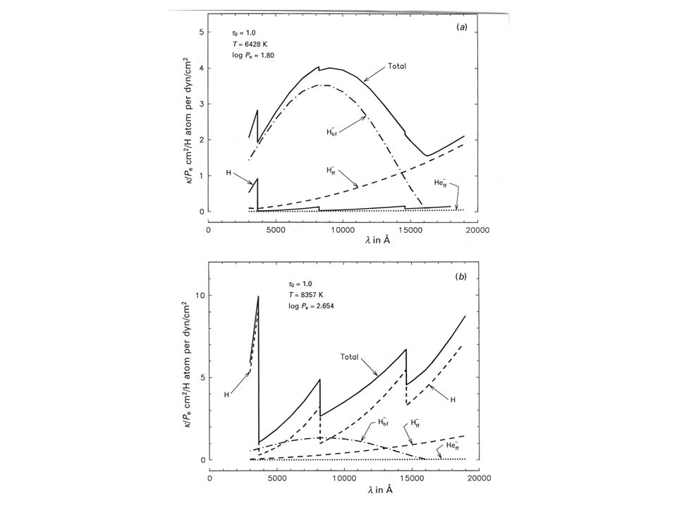
31. III. Total Absorption Coefficient for Hydrogen total bound-free free-free

32. IV. The Negative Hydrogen Ion The hydrogen atom is capable of holding a second electron in a bound state. The ionization of the extra electron requires 0.754 eV All photons with  < 16444 Ang have sufficient energy to ionize H – back to neutral H Very important opacity for T eff < 6000 K Where does this extra electron come from? Metals!

33. IV. The Negative Hydrogen Ion For T eff > 6000 K, H – too frequently ionized to be an effective absorber For T eff < 6000 K, H – very important For T eff < 4000 K, no longer effective because there are no more free electrons

34. IV. The Negative Hydrogen Ion The bound free absorption coefficient can be expressed by the following polynomial  bf = a 0 + a 1 + a 2 2 + a 3 3 + a 4 4 + a 5 5 + a 6 6 a 0 = 1.99654 a 1 = –1.18267 × 10 –5 a 2 = 2.64243 × 10 –6 a 3 = –4.40524 × 10 –10 a 4 = 3.23992× 10 –14 a 5 = –1.39568 × 10 –10 a 6 = 2.78701 × 10 –23 is in Angstroms

35. IV. The Negative Hydrogen Ion: Bound-Free Wavelength (angstroms)  bf, 10 –18 cm 2 per H – ion

36. IV. The Negative Hydrogen Ion: bound-free The H – ionization is given by the Saha equation log N(H) N(H – ) = –log P e – 5040 T I +2.5 log T + 0.1248 in eV  (H bf – ) = 4.158 × 10 –10  bf P e  2 5 10 0.754  u 0 (T) = 1, u 1 (T) = 2

37. IV. The Negative Hydrogen Ion: free-free  (H ff – ) = P e  ff = 10 –26 × P e 10 f 0 +f 1 log  +f 2 log2  f 0 = –2.2763–1.685 log +0.766 log 2 –0.0533464 log 3 f 1 = 15.2827–9.2846 log +1.99381 log 2 –0.142631 log 3 f 3 = –197.789+190.266 log –67.9775 log 2 +10.6913 log 3 –0.625151 log 4

38. IV. The Negative Hydrogen Ion: Total bound-free free-free

39. V. The Negative Helium ion The bound–free absorption is neglible, but free-free can be important in the atmospheres of cool stars

40. VI. Metals In the visible a minor opacity source because they are not many around Contribute indirectly by providing electrons In the visible  (metals) ~ 1%  (H bf – ) A different story in the ultraviolet where the opacity is dominated by metals

41. VI. Metals The absorption coefficient for metals dominate in the ultraviolet

42. VII. Electron (Thompson) Scattering Important in hot stars where H is ionized Only true „grey“ opacity source since it does not depend on wavelength Phase function for scattering ~ 1 + cos  Stellar atmosphere people assume average phase ~ 0

43. The absorption coefficient is wavelength independent:  e = 88 3 ( ( e2e2 mc 2 2 = 0.6648 x 10 –24 cm 2 /electron The absorption per hydrogen atom:  (e) = eNeeNe NHNH ePeePe PHPH = P H = Partial pressure of Hydrogen VII. Electron (Thompson) Scattering

44. P H is related to the gas and electron pressure as follows: N =  N j + N e =  NHNH A j + N e N j particles of the jth element per cubic cm and A j = N j /N H Solving for N H NHNH = N–NeN–Ne  AjAj PHPH = Pg–PePg–Pe  AjAj VII. Electron (Thompson) Scattering

45.  (e) = Electron scattering is important in O and Early B stars P g – P e ePeePe  AjAj If hydrogen dominates their composition P e = 0.5P g  (e) = ee  AjAj Independent of pressure VII. Electron (Thompson) Scattering

46. P e /P Tot T eff P Tot = P e + P g 0.5

47. VIII. Other Sources of Opacity H 2 (neutral) has no significant absorption in the visible H 2 +, H 2 – do have significant absorption H 2 + (bf) important in the ultraviolet, in A-type stars it is ~ 10% of H – bound-free opacity Peaks in opacity around  ≈ 1100 Å, is dominated by the Balmer continuum below 3600 Å in most stars H 2 – (free-free) important in the infrared (cool stars) and fills the opacity minimum of H – at 16400 Å H 2 molecules

48. bound-free free-free

49. VIII. Other Sources of Opacity Important only in O and B-type stars He II (bound-free) is hydrogenic → multiply hydrogen cross sections by Z 4 or 16. He I (bound-free), He II (bound-free)

50. VIII. Other Sources of Opacity Important in cool stars Scattering by molecules and atoms Has a 1/ 4 dependence Rayleigh Scattering

51. VIII. Other Sources of Opacity Molecules and ions: CN –, C 2 –, H 2, He, N 2, O 2, TiO,.... Cool Stars Basically Cool Stars are a mess and only for the bravest theoretical astrophysicist

52. IX. Summary of Continuous Opacities Spectral Type Dominant opacity O–BElectron scattering, He I,II (b-f), H(f-f) B–AH I: b-f, f-f He II: b-f, some electron scattering A–Fequal contributions from H I (b-b) H I (f-f), H – (b-f, f-f) G–K H I (b-f), H – (b-f, f-f), Rayleigh Scattering off H I

53. IX. Summary of Continuous Opacities Spectral Type Dominant opacity K–Early M H – (b-f, f-f), Rayleigh scattering (UV) off H I and H 2, molecular opacities (line blanketing) M:Molecules and neutral atoms, H – (b-f, f-f), Rayleigh scattering off other molecules

56. He II/He III ionization zone Contraction During compression He II ionized to He III, He III has a higher opacity. This blocks radiation causing star to expand Cepheid Pulsations are due to an opacity effect: During expansion He zone cools, He III recombines, opacity decreases allowing photons to escape. Star then contracts under gravity. Expansion

57. Most pulsating stars can be explained by opacity effects