1. Chapter 12 Graphs and the Derivative Abbas Masum

2. Chapter 4 Review  Find f’(x) if f(x) = (3x – 2x 2 ) 3  3(3x – 2x 2 ) 2 (3 – 4x)

3. Review

4.  Find f’(x) if

5. Continued

6. The graph of y = f (x): increases on ( – ∞, – 3), decreases on ( – 3, 3), increases on (3, ∞). Increasing, Decreasing, and Constant Functions (3, – 4) x y ( – 3, 6) Increasing & Decreasing Functions A function can be increasing, decreasing, or constant

7. Increasing/Decreasing

8. Increasing/Decreasing Test

9. Critical Numbers The derivative can change signs (positive to negative or vice versa) where f’(c) = 0 or where f”(c) DNE. A critical point is a point whose x-coordinate is the critical number.

10. Applying the Test FFind the intervals where the function f(x)=x3+3x2-9x+4 is increasing/decreasing and graph. 11. Find the critical numbers by setting f’(x) = 0 and solving: f’(x) = 3x2 + 6x – 9 0 = 3(x2 + 2x – 3) 0 = 3(x + 3)(x - 1) x = -3, 1 The tangent line is horizontal at x = -3, 1

11. Test  Mark the critical points on a number line and choose test points in each interval

12. Test EEvaluate the test points in f’(x): 3(x+3)(x-1) ff’(-4) = (+)(-)(-) = + ff’(0) = (+)(+)(-) = - ff’(2) = (+)(+)(+) = +

13. To Graph  To graph the function, plug the critical points into f(x) to find the ordered pairs:  f(x)=x 3 +3x 2 -9x+4  f(-3) = 31  f(1) = -1

14. Relative (or Local) Extrema

15. The First Derivative Test

16. First Derivative Test

17. You Do FFind the relative extrema as well as where the function is increasing and decreasing and graph. ff(x) = 2x 3 – 3x 2 – 72x + 15 CCritical points: x = 4, -3

19. Higher Derivatives, Concavity, the Second Derivative Test  Given f(x) = x 4 + 2x 3 – 5x + 7, find  f’(x) =  f”(x) =  f’”(x) =  f (4) (x) = 4x 3 + 6x 2 - 5 12x 2 + 12x 24x + 12 24

20. Find the 1st and 2nd Derivatives  f(x) = 4x(ln x)  f’(x) =  f”(x) =

21. Position Function AA car, moving in a straight line, starting at time, t, is given by s(t) = t 3 – 2t 2 – 7t + 9. Find the velocity and acceleration vv(t) = s’(t) = 3t 2 – 4t – 7 aa(t) = v’(t) = s”(t) = 6t - 4

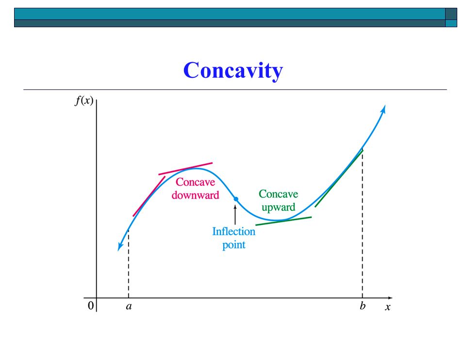
22. Concavity

24. Test for Concavity

25. 2nd Derivative Test By setting f”(x) = 0, you can fin the possible points of inflection (where the concavity changes).

26. Curve Sketching 1. Note any restrictions in the domain (dividing by 0, square root of a negative number…) 2. Find the y-intercept (and x-intercept if it can be done easily). 3. Note any asymptotes (vertical asymptotes occur when the denominator = 0, horizontal asymptotes can be found by evaluating x as x →∞ or as x →-∞

27. Example 1: Graph the function f given by and find the relative extrema. 1 st find f (x) and f  (x).

28. Example 1 (continued): 2 nd solve f (x) = 0. Thus, x = –3 and x = 1 are critical values.

29. Example 1 (continued): 3 rd use the Second Derivative Test with –3 and 1. Lastly, find the values of f (x) at –3 and 1. So, (–3, 14) is a relative maximum and (1, –18) is a relative minimum.

30. Example 1 (concluded): Then, by calculating and plotting a few more points, we can make a sketch of f (x), as shown below.

31. Strategy for Sketching Graphs: a) Derivatives and Domain. Find f (x) and f  (x). Note the domain of f. b) Find the y-intercept. c) Find any asymptotes. d)Critical values of f. Find the critical values by solving f (x) = 0 and finding where f (x) does not exist. Find the function values at these points.

32. Strategy for Sketching Graphs (continued): e) Increasing and/or decreasing; relative extrema. Substitute each critical value, x0, from step (b) into f  (x) and apply the Second Derivative Test. f) Inflection Points. Determine candidates for inflection points by finding where f  (x) = 0 or where f  (x) does not exist. Find the function values at these points.

33. Strategy for Sketching Graphs (concluded): g) Concavity. Use the candidates for inflection points from step (d) to define intervals. Use the relative extrema from step (b) to determine where the graph is concave up and where it is concave down. h) Sketch the graph. Sketch the graph using the information from steps (a) – (e), calculating and plotting extra points as needed.

34. Example 3: Find the relative extrema of the function f given by and sketch the graph. a) Derivatives and Domain. The domain of f is all real numbers.

35. Example 3 (continued): b) Critical values of f. And we have f (–1) = 4 and f (1) = 0.

36. Example 3 (continued): c) Increasing and/or Decreasing; relative extrema. So (–1, 4) is a relative maximum, and f (x) is increasing on (–∞, –1] and decreasing on [–1, 1]. The graph is also concave down at the point (–1, 4). So (1, 0) is a relative minimum, and f (x) is decreasing on [–1, 1] and increasing on [1, ∞). The graph is also concave up at the point (1, 0).

37. Example 3 (continued): d) Inflection Points. And we have f (0) = 2. e) Concavity. From step (c), we can conclude that f is concave down on the interval (–∞, 0) and concave up on (0, ∞).

38. Example 3 (concluded) f) Sketch the graph. Using the points from steps (a) – (e), the graph follows.

39. Example 5: Graph the function f given by List the coordinates of any extreme points and points of inflection. State where the function is increasing or decreasing, as well as where it is concave up or concave down.

40. Example 5 (continued) a) Derivatives and Domain. The domain of f is all real numbers.

41. Example 5 (continued) b) Critical values. Since f (x) is never 0, the only critical value is where f (x) does not exist. Thus, we set its denominator equal to zero. And, we have

42. Example 5 (continued) c) Increasing and/or decreasing; relative extrema. Since f  (x) does not exist, the Second Derivative Test fails. Instead, we use the First Derivative Test.

43. Example 5 (continued) c) Increasing and/or decreasing; relative extrema (continued). Selecting 2 and 3 as test values on either side of Since f’(x) is positive on both sides of is not an extremum.

44. Example 5 (continued) d) Inflection points. Since f  (x) is never 0, we only need to find where f  (x) does not exist. And, since f  (x) cannot exist where f (x) does not exist, we know from step (b) that a possible inflection point is ( 1).

45. Example 5 (continued) e) Concavity. Again, using 2 and 3 as test points on either side of Thus, is a point of inflection.

46. Example 5 (concluded) f) Sketch the graph. Using the information in steps (a) – (e), the graph follows.

47. In Summary Curve Sketching 4. Find f’(x). Locate critical points by solving f’(x) = 0. 5. Find f”(x). Locate points of inflection by solving f”(x) = 0. Determine concavity. 6. Plot points. 7. Connect the points with a smooth curve. Points are not connected if the function is not defined at a certain point.

48. Example GGraph f(x) = 2x 3 – 3x 2 – 12x + 1 YY-intercept is (0,1) CCritical points: f’(x) = 6x 2 – 6x – 12 x = 2, -1

49. GGraph f(x) = 2x 3 – 3x 2 – 12x + 1 YY-intercept is (0,1) CCritical points: f’(x) = 6x 2 – 6x – 12 x = 2, -1 PPoints of inflection: f”(x) = 12x – 6 x = ½

51. GGraph f(x) = 2x 3 – 3x 2 – 12x + 1 YY-intercept is (0,1) CCritical points: f’(x) = 6x 2 – 6x – 12 x = 2, -1 PPoints of inflection: f”(x) = 12x – 6 x = - ½ PPlug critical points into f(x) to find y’s f(2) = -19, f(-1) = 8

52. Graph

53. 12.2 Second Derivative and Graphs

54. “If we think the derivative as a rate of change, then the second derivative is the rate of change of the rate of change” * The second derivative is the derivative of the derivative

55. Compare f(x) and g(x) Both are increasing functions but they don’t look quite the same.

56. Compare f’(x) and g’(x) Both f’(x) and g’(x) are positive, however, f’(x) – the slope of the tangent line - is increasing but g’(x) is decreasing

57. Concavity Tests Theorem. The graph of a function f is concave upward on the interval (a,b) if f ’(x) is increasing on (a,b), and is concave downward on the interval (a,b) if f ’(x) is decreasing on (a,b). For y = f (x), the second derivative of f, provided it exists, is the derivative of the first derivative: Theorem. The graph of a function f is concave upward on the interval (a,b) if f ’’(x) is positive on (a,b), and is concave downward on the interval (a,b) if f ’’(x) is negative on (a,b).

58. Relationship between F and F’’ F: increasing on (-∞,-1) and (1,∞) decreasing on (-1,1) So F’ > 0 on (-∞,-1) and (1,∞) F’ < 0 on (-1,1) F’: decreasing on (- ∞, 0) increasing on (0, ∞) So F’’ < 0 on (- ∞, 0) F’’ > 0 on (0, ∞) F: concave down (- ∞, 0) concave up (0, ∞) So F’’ < 0 on (- ∞, 0) F’’ > 0 on (0, ∞) F’’(x) F(x) F’(x)

60. Concavity Concave down Concave up

61. up down up Concavity

62. Example 1 Determine the intervals on which the graph is concave upward and the intervals on which it’s concave downward. A) f(x) = -e -x Domain (-∞∞), no critical point f’(x) = -e -x (-1) = e -x f’’(x) = e -x (-1) = -e -x Test some numbers in the domain (review section 12.1 if you forgot), we will see that f’’ is always negative. Therefore, the graph of f(x) is concave downward on (-∞∞)

63. Example 1 (continue) Determine the intervals on which the graph is concave upward and the intervals on which it’s concave downward. B) f(x) = ln (1/x) (that should equal ln 1 – lnx) Domain (0,∞), no critical point f’(x) = -1/x = -x -1 f’’(x) = x -2 = 1/x 2 Test some numbers in the domain, we will see that f’’ is always positive. Therefore, the graph of f(x) is concave upward on (0,∞)

64. Example 1 (continue) Determine the intervals on which the graph is concave upward and the intervals on which it’s concave downward. C) f(x) = x 1/3 Domain (-∞,∞), critical value is x = 0 Since there is a critical point, we want to test some points on the left of 0 and some on the right of 0. We will see that f’’ is always positive on the left of 0 and always negative on the right of 0. Therefore, the graph of f(x) is concave upward on (-∞, 0) and concave downward on (0, ∞). Note that this graph changes from concave upward to concave downward at (0,0). This point is called an inflection point.

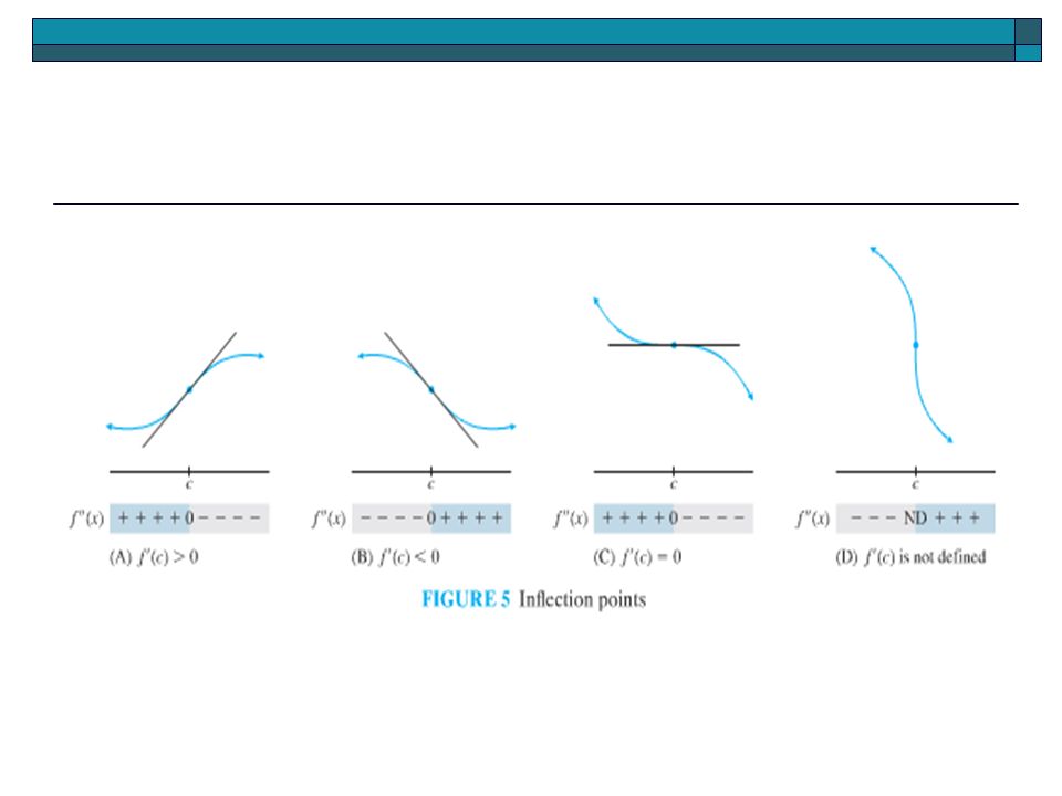
65. Inflection Points An inflection point is a point on the graph where the concavity changes from upward to downward or downward to upward. This means that if f ’’(x) exists in a neighborhood of an inflection point, then it must change sign at that point. Theorem 1. If y = f (x) is continuous on (a,b) and has an inflection point at x = c, then either f ’’(c) = 0 or f ’’(c) does not exist.

67. Example 2 Find the inflection point(s) of f(x) = x 3 – 9x 2 +24x -10 F’(x) = 3x 2 – 18x + 24 F’’(x) = 6x – 18 = 0 6(x-3) = 0 x = 3 +0--F’’ 432x Concave downConcave up Therefore 3 is the infection point of f(x) Note: It’s important to do this test because the second derivative must change sign in order for the graph to have an inflection point.

68. Example 3: A special case Find the inflection point(s) of f(x) = x 4 F’(x) = 4x 3 F’’(x) = 12x 2 = 0 x = 0 +0+F’’ 10x Concave up Therefore 0 is not the inflection point of f(x) There is no inflection point for this graph

69. Example 4 Find the inflection point(s) of f(x) = ln(x 2 - 2x + 5) x = -1 and x =3 + 0 0 3 -0-F’’ 4-2x Concave down Concave up Therefore there are two inflection points at x= -1 and x=3 Concave down

70. Example 5 The given graph shows the graph of the derivative function f’(x). Discuss the graph of f and sketch a possible graph of f. F’(x) Local maximumX-interceptX=2 Increasing Concave up positive increasing (-1,1) Inflection pointLocal maximumX=1 Increasing Concave down Positive decreasing (1,2) Decreasing Concave down Negative decreasing (2, ∞) Inflection pointLocal minimumX= -1 Increasing Concave down Positive Decreasing (-∞,-1) F(x)F’(x)x

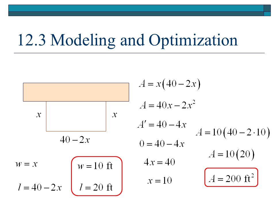
71. A Classic Problem You have 40 feet of fence to enclose a rectangular garden along the side of a barn. What is the maximum area that you can enclose? 12.3 Modeling and Optimization

73. To find the maximum (or minimum) value of a function: 12.3 Modeling and Optimization 1.Understand the Problem. 2.Develop a Mathematical Model. 3.Graph the Function. 4.Identify Critical Points and Endpoints. 5.Solve the Mathematical Model. 6.Interpret the Solution.

74. What dimensions for a one liter cylindrical can will use the least amount of material? We can minimize the material by minimizing the area. area of ends lateral area We need another equation that relates r and h: 12.3 Modeling and Optimization

75. area of ends lateral area 12.3 Modeling and Optimization

76. Find the radius and height of the right-circular cylinder of largest volume that can be inscribed in a right-circular cone with radius 6 in. and height 10 in. h r 10 in 6 in

77. 12.3 Modeling and Optimization h r 10 in 6 in The formula for the volume of the cylinder is To eliminate one variable, we need to find a relationship between r and h. 6 h 10-h r 10

78. 12.3 Modeling and Optimization h r 10 in 6 in

79. 12.3 Modeling and Optimization h r 10 in 6 in Check critical points and endpoints. r = 0, V = 0 r = 4 V = 160  /3 r = 6 V = 0 The cylinder will have a maximum volume when r = 4 in. and h = 10/3 in.

80. Determine the point on the curve y = x 2 that is closest to the point (18, 0). 12.3 Modeling and Optimization Substitute for x

81. Determine the point on the curve y = x 2 that is closest to the point (18, 0). 12.3 Modeling and Optimization

82. Determine the point on the curve y = x 2 that is closest to the point (18, 0). 12.3 Modeling and Optimization 2 - 0 +

83. If the end points could be the maximum or minimum, you have to check. Notes: If the function that you want to optimize has more than one variable, use substitution to rewrite the function. If you are not sure that the extreme you’ve found is a maximum or a minimum, you have to check. 12.3 Modeling and Optimization

84. Applying Our Concepts  We know about max and min …  Now how can we use those principles?

86. Use the Strategy  What is the quantity to be optimized? The volume  What are the measurements (in terms of x)?  What is the variable which will manipulated to determine the optimum volume?  Now use calculus principles x 30” 60”

87. Guidelines for Solving Applied Minimum and Maximum Problems

88. Optimization Maximizing or minimizing a quantity based on a given situation Requires two equations: Primary Equation what is being maximized or minimized Secondary Equation gives a relationship between variables

89. 1.An open box having a square base and a surface area of 108 square inches is to have a maximum volume. Find its dimensions. Primary Secondary Intervals: Test values: V ’(test pt) V(x) rel max Domain of x will range from x being as small as possible to x as large as possible. Smallest (x is near zero) Largest (y is near zero) Dimensions: 6 in x 6 in x 3 in

90. 2.Find the point on that is closest to (0,3). Primary Secondary Intervals: Test values: d ’(test pt) d(x) rel min ***The value of the root will be smallest when what is inside the root is smallest. rel max rel min Minimize distance

91. 2.A rectangular page is to contain 24 square inches of print. The margins at the top and bottom are 1.5 inches. The margins on each side are 1 inch. What should the dimensions of the print be to use the least paper?

92. Primary Secondary Intervals: Test values: A ’(test pt) A(x) rel min Smallest (x is near zero) Largest (y is near zero) Print dimensions: 6 in x 4 in Page dimensions: 9 in x 6 in

93. Example  A company needs to construct a cylindrical container that will hold 100cm 3. The cost for the top and bottom of the can is 3 times the cost for the sides. What dimensions are necessary to minimize the cost. r h

94. Minimizing Cost Domain: r>0

95. Minimizing Cost Concave up – Relative min The container will have a radius of 1.744 cm and a height of 10.464 cm 1.744 0 - - - + + + + + C' changes from neg. to pos.  Rel. min