1. Predicate Calculus CS 270 Math Foundations of Computer Science Jeremy Johnson Presentation uses material from Huth and Ryan, Logic in Computer Science: Modelling and Reasoning about Systems, 2nd Edition

2. Outline 1.Motivation (program specification & derivation) 1.Variables, quantifiers and predicates 2.Syntax 1.Terms and formulas 2.Quantifiers, scope and substitution 3.Rules of natural deduction for quantifiers 4.Semantics 1.Models and semantic entailment 5.Undecidability and limitations

3. Hamiltonian Path G = (V,E) is an undirected graph with nodes V = {0,1,…,n-1} and edges E  V  V V = {0,1,2} E = {(0,1),(1,2)} edge(0,1), edge(1,0), edge(1,2), edge(2,1) 1 02

4. Hamiltonian Path A Hamiltonian path is a sequence of n nodes, where n = |V| where each node is visited exactly once (i.e. a permutation of the nodes) following edges 1 02 0  1  2 or 2  1  0

5. Hamiltonian Path path(i,j) is true when the jth node in the path is in the ith location Hamiltonian paths path(0,0), path(1,1), path(2,2) path(0,2), path(1,1), path(2,0) Not Hamiltonian paths path(0,0), path(1,2), path(2,1) path(0,0), path(0,1), path(1,1), path(2,2) path(0,0), path(1,1), path(1,0), path(2,2) 1 02

6. Hamiltonian Path Constraints Every node occurs exactly once in the path  j  i path(i,j)  j  i  k path(i,j)  path(k,j)  i = k Every location has exactly one node  i  j path(i,j)  i  j  k path(i,j)  path(i,k)  j = k Adjacent nodes must be connected by an edge  i  j  k (i<n-1)  (path(i,j)  path(i+1,k)  edge(j,k))

7. Simplification Every node occurs exactly once in the path  j  i  k path(i,j)  path(k,j)  i = k  j  i  k (i  k   (path(i,j)  path(k,j))  j  i  k (i  k)   path(i,j)   path(k,j)  j  i  k (i < k)   path(i,j)   path(k,j)

8. Simplification Adjacent nodes must be connected by an edge  i  j  k (i<n-1)  ((path(i,j)  path(i+1,k))  edge(j,k))  i  j  k (i<n-1)  (  edge(j,k)   (path(i,j)  path(i+1,k)))  i  j  k (i<n-1)  (  edge(j,k)  (  path(i,j)   path(i+1,k)))  i  j  k ((i<n-1) &  edge(j,k))  (  path(i,j)   path(i+1,k)))

9. Conversion to SAT  j  i path(i,j)  j=0..n-1  i=0..n-1 P ij  j  i  k (i < k)   path(i,j)   path(k,j)  j=0..n-1  i=0..n-1  k=i+1..n-1  P ij   P kj  i  j  k ((i<n-1) &  edge(j,k))  path(i,j)  path(i+1,k))  i=0..n-2  (j,k)  E  P ij   P i+1,k

10. Example 1 Every student is younger than some instructor  x ( S(x)   y(I(y)  Y(x,y) ) S(x) : x is a student I(x) : is an instructor Y(x,y) : x is younger than y

11. Example 2 Not all birds can fly   x ( B(x)  F(x) )  x ( (B(x)   F(x) ) B(x) : x is a bird F(x) : x can fly Semantically equivalent formulas

12. Example 3 Every child is younger than its mother  x  y ( C(x)  M(y,x)  Y(x,y) ) C(x) : x is child M(x,y) : x is y’s mother Y(x,y) : x is younger than y  x ( C(x)  Y(x,m(x)) m(x) : function for mother of x

13. Example 4 Andy and Paul have the same maternal grandmother  x  y  u  v ( M(x,y)  M(y,a)  M(u,v)  M(v,p)  x = u ) m(m(a)) = m(m(p)) a, b : variables for Andy and Paul = : binary predicate

14. Example 5 Everyone has a mother  x  y ( M(y,x) )  x  y ( M(y,x) ) [ not equivalent ] Everyone has exactly one mother  x  y ( M(y,x)   z (M(z,x)  z = y )

15. Example 6 Some people have more than one brother  x  y1  y2 ( B(y1,x)  B(y2,x)   (y1 = y2) )

16. Comparison to Propositional Calculus

17. Terms Terms are made up of variables, constants, and functions Term ::= Variable If c is a nullary function c is a term If t 1,…,t n are terms and f is an n-ary function then f(t 1,…,t n ) is a term

18. Formulas Formula ::= P is a predicate and t 1,…,t n are terms then P(t 1,…,t n ) is a formula If  is a formula  is a formula If  1 and  2 are formulas,  1   2,  1   2,  1   2 are formulas If  is a formula and x is a variable  x  and  x  are formulas

19. Parse Trees  x ( ( P(x)  Q(x) )  S(x,y) ) xx  S  xy P Q x x

20. Free and Bound Variables An occurrence of x in  is free if it is a leaf node in the parse tree for  with no quantifier as an ancestor xx  S  xy P Q x x xx  P Q x x    P x Q y

21. Substitution Given a variable x, a term t and a formula ,  [t/x] is the formula obtained by replacing each free occurrence of x by t xx  P Q x x   P x Q y  xx  P Q x x   P f Q y  x y  [f(x,y)/x]

22. Variable Capture t is free for x in  if no free x occurs in  in the scope of any quantifier for any variable y occurring in t. yy  S x  P Q x y

23. Variable Capture t is free for x in  if no free x occurs in  in the scope of any quantifier for any variable y occurring in t. yy  S x  P Q y f y y

24. Equality Rules Introduction Rule Elimination Rule = i t = t t 1 = t 2  [t 1 /x] =e  [t 2 /x]

25. Equivalence Relation 1premise 2=i 3=e 1,2 1premise 2 3=e 2,1

26. Conjunction Rules Introduction Rule Elimination Rule    i     e1      e2 

27. Universal Quantification Rules Introduction Rule Elimination Rule  x i  x   x e  [t/x] x 0 …  [x 0 /x]

28. Illegal Substitution Leads to False Reasoning  x   =  y (x < y)  [y/x] =  y (y < y) y is not free for x in 

29. Example Proof 1premise 2 3 x 0 P(x 0 )  Q(x 0 ) 4P(x 0 ) 5Q(x 0 )  e3,4 6

30. Disjunction Rules Introduction Rule Elimination Rule (proof by case analysis)   i1     e    i2    …… ……

31. Existential Quantification Rules Introduction Rule Elimination Rule (proof by case analysis)  [t/x]  x i  x   e  x 0  [x 0 /x] … 

32. Example Proof 1premise 2 3 x 0 P(x 0 )  Q(x 0 ) assumption 4 5Q(x 0 )  e 2 3 6 7 P(x 0 )  e 1 3 8 P(x 0 )  R(x 0 )  i7,6 9 10

33. Quantifier Equivalences

35. De Morgan’s Law 1premise 2assumption 3 4  i 1 3 5  e4,2 6  e 3-5 7assumption 8  i 2 7 9 10  e 7-9 11 12 13  e 2-12

36. Generalized De Morgan’s Law 1  x P(x) premise 2assumption 3x0x0 4 5 6 7  e 4-6 8 9 10  x  P(x)  e 2-9

37. Generalized De Morgan’s Law 1  x  premise 2assumption 3x0x0 4 5 6 7  e 4-6 8 9 10  x  e 2-9

38. Exercise

39. Models Let F be a set of functions and P a set of predicates. A model M for (F,P) consists of A non-empty set A [universe] of concrete values For each nullary f  F an element of A = f M For each n-ary f  F a function f M : A n  A For each n-ary P  P a subset P M  A n

40. Example 1 F = {i} and P = {R,F} i a constant function, R binary and F unary predicates Model – A set of states, initial state i, state transitions R, final states F A = {a,b,c} i M = a R M = {(a,a),(a,b),(a,c),(b,c), (c,c)} F M = {b,c}

41. Example 1  y R(i,y)  F(i)  x  y  z (R(x,y)  R(x,z)  y = z )  x  y R(x,y)

42. Example 2 F = {e,  } and P = {  } e a constant function,  a binary function,  a binary predicate Model – string prefix A = {binary strings} e M = ,  M concatenation,  M prefix ordering [011 is a prefix of 011001

43. Example 2  x ((x  x  e)  x  e  x))  x  y (y  x)  y  x (y  x)  x  y  z ((x  y)  (y  z)  (x  z))  x  y  z ((x  y)  (x  z  y  z))

44. Satisfaction

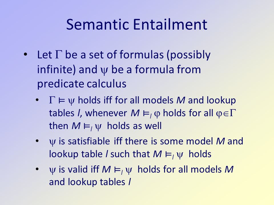
46. Semantic Entailment

48. Soundness and Completeness

49. Post Correspondence Given a finite sequence (s 1,t 1 ),…,(s k,t k ) of pairs of binary strings. Is there a sequence of indices i 1,i 2,…,i n such that s i 1  s i n = t i 1  t i n Example s 1 = 1, s 2 = 10, s 3 = 011 t 1 = 101, t 2 = 00, t 3 = 11 Solution (1,3,2,3) 101110011

50. Undecidability

51. Consequences of Undecidability

52. Proof

57. Reachabilty When modeling systems via states and state transitions, we want to show that a “bad” state can not be reached from a “good” state. Given nodes n and n’ in a directed graph, is there a finite path of transitions from n to n’. s0 s1 s3 s2 A = {s0,s1,s2,s3} R M = {(s0,s1), (s1,s0), (s1,s1),(s1,s2), (s2,s0),(s3,s0),(s3,s2)}

58. Compactness Theorem Let  be a set of sentences of predicate calculus. If all finite subsets of  are satisfiable, then so is . Proof – uses soundness and completeness and finite length of proofs.

59. Reachability is Not Expressible Can reachability be expressed in predicate calculus? u=v   x (R(u,x)  R(x,v))   x 1  x 2 (R(u,x 1 )  R(x 1,x 2 )  R(x 2,v))  … This is infinite The answer is no! Proof follows from compactness theorem.

60. Reachability is Not Expressible Theorem. There is no predicate-logic formula  with u and v as its only free variables and R its only predicate such that  holds in directed graphs iff there is a path from u to v. Proof. By contradiction. Suppose there is such a formula. Let  n be the formula expressing that there is a path from c to c’  n =  x 1 …  x n-1 (R(c,x 1 )  …  R(x n-1,c)).

61. Reachability is Not Expressible Proof. By contradiction. Suppose there is such a formula . Let  n be the formula expressing that there is a path from c to c’  n =  x 1 …  x n-1 (R(c,x 1 )  …  R(x n-1,c)).  = {   i | I  0}   [c/u][c’/v] is unsatisfiable, but any finite subset is satisfiable. By compactness this leads to a contradiction and hence there is no such .

62. Reachability via HOL

63. Obtain formula for the existence of a path from u to v by negating previous formula (use DeMorgan’s law)  P  x  y  z (  C 1   C 2   C 3   C 4 ) If both  and  can range over predicates then second order logic.