1. ATMIYA INSTITUTE OF TECHNOLOGY & SCIENCE MECHANICAL DEPARTMENT 5th SEMESTER
GOVERNOR
PREPARED BY:
YASH SHAH( )
KAUMIL SHAH ( )

2. CONTENTS NECESSITY OF GOVERNOR CLASSIFICATION OF GOVERNORS
WORKING PRINCIPLE OF CENTRIFUGAL GOVERNOR
CONCEPT OF CONTROL FORCE
CONTROL FORCE DIAGRAM

3. The Original Governor
James Watt’s
Flyball Governor
Used to prevent steam engines from overheating while responding to the applied loads.

4. INTRODUCTION
The function of governor is to regulate the speed of an engine when there are variation in the load.
Eg. When the load on an engine increases, its speed decreases, therefore it is necessary to increase the supply of working fluid & vice-versa. Thus, Governor automatically controls the speed under varying load.
Types of Governors:
The governors may broadly be classified as
Centrifugal governors
Inertia governors

5. Modern Governor

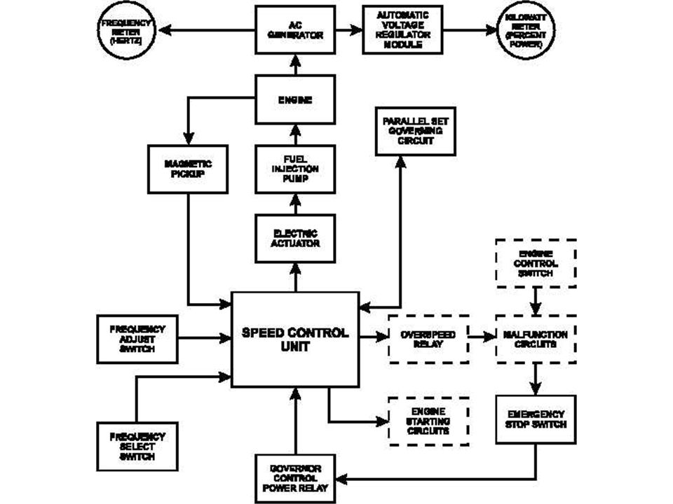
6. Why Use an Electronic Governor?
Allows for very precise governing
Requires very limited amount of moving parts
Can fit in small areas
Easy to adjust for changes in application
Interfaces easily with other controlling devices

7. Why Use a Mechanical Governor?
Could be less expensive
Can use in wide range of conditions
Marine Applications
Extreme Temperatures
Usually easier to troubleshoot
More transparent

8. Mechanical Governor Shortcomings
Have a delayed response time called “droop”
This delay in response time induces something called “hunting”
Can be thought of in terms of overshoot and over/under damping
Can tune a mechanical system to minimize hunting using additional external mechanical governors

9. Simple MatLAB Simulation

10. CLASSIFICATION OF GOVERNORS
Centrifugal governor
Pendulum type
Loaded type
Watt governor
Dead weight governor
Spring controlled governor
Porter governor
Proell governor
Pickering governor
Hartung governor
Wilson - Hartnel governor
Hartnell governor

11. CENTRIFUGAL GOVERNORS
The centrifugal governors are based on the balancing of centrifugal force on the rotating balls for an equal and opposite radial force, known as the controlling force.
It consist of two balls of equal mass, which are attached to the arms as shown in fig. These balls are known as governor balls or fly balls.

13. WORKING PRINCIPLE OF CENTRIFUGAL GOVERNOR
when the load on the engine increases, the engine and the governor speed decreases.
This results in the decrease of centrifugal force on the balls. Hence the ball moves inward & sleeve moves downwards.
The downward movement of sleeve operates a throttle valve at the other end of the bell rank lever to increase the supply of working fluid and thus the speed of engine is increased.
In this case the extra power output is provided to balance the increased load.

14. When the load on the engine decreases, the engine and governor speed increased, which results in the increase of centrifugal force on the balls.
Thus the ball move outwards and sleeve rises upwards.
This upward movement of sleeve reduces the supply of the working fluid and hence the speed is decreased.
In this case power output is reduced.

15. CONCEPT OF CONTROL FORCE
The resultant external force which controls the movement of the ball and acts along the radial line towards the axis is called controlling force. This force acts at the centre of the ball. It is equal and acts opposite to the direction of centrifugal force. The controlling force ‘F’ = m w2 r
Stability of Spring-controlled Governors Figure 5.8 shows the controlling force curves for stable, isochronous and unstable spring controlled governors. The controlling force curve is approximately straight line for spring controlled governors. As controlling force curve represents the variation of controlling force ‘F’ with radius of rotation ‘r’, hence, straight line equation can be,F=ar+b where a and b are constants. In the above equation b may be +ve, or –ve or zero.

16. CONTROL FORCE DIAGRAM

18. Thank you !!!