1. Financing of Public Good by Taxation in a General Equilibrium Economy: Theory and Experimental Evidence Shyam Sunder, Yale University (with Juergen Huber and Martin Shubik) Max Planck Institute for Collective Goods Bonn, Germany, July 14, 2011

2. Importance and Financing of Public Goods Public goods are important; how do and should societies finance them? Experimental work, mostly voluntary anonymous contributions Ledyard survey of pre-1995 literature; more recently Fehr and Gächter (2000); Gunnthorsdottir, Houser and McCabe (2007); Brandts and Schram (2001); Palfrey and Prisbrey (1997) High initial contributions ), e.g., 50 percent of optimal), tend to decline towards 10 percent over time and experience

3. Financing Public Goods in General Equilibrium We modify a general equilibrium model of the economy to include government and a full process description of agents playing both economic (market) and political (voting) roles. We use a process oriented strategic market game in which the provision of public goods is financed through taxation on private income. The unique equilibrium solution for any tax rate yields an optimal consumption/investment policy for each individual. A general dynamic programming analysis of our basic model enables us to solve for an optimal rate of taxation for society as a whole using symmetry of the agents in the model. Simplification some fundamental features of government control of taxation, and public debt creation to provide valued public services. Hatzipanayotou and Michael (2001) who deal with public goods, tax policies and unemployment in LDCs is closer to the spirit of our own approach where institutional structure plays an important role in the economy.

4. All equations of motion are specified in a complete dynamic model of the economy. Although the investigation focuses on equilibrium outcomes, our model is defined for all feasible outcomes in the economy, as is shown in Figure xxx, in Appendix A for the specific parameters and functional forms used here. As a reasonably general solution to the dynamic programming model has been provided elsewhere (KSS 2011) using an Excel spreadsheet it is possible to illustrate the full payoff set and the optimum for any model in the large class consistent with the general model.

5. Model

6. Experimental Design 2x2 treatment We examine the model in a laboratory setting when – The economy starts from an optimum level of public good, and – When it starts at 50 percent of the optimum level The efficiency of the outcomes of the economy will be compared – When the rate of taxation is exogenously fixed at the theoretical optimal level, which is practical only in a hypothetical world of an omniscient government; and – When the rate of taxation can be adjusted by the political process that moves on a longer time scale than the day-to-day economic process (tax rate set to the median of the individual proposals) Compare the outcomes of the human-subject against two benchmarks: – The general equilibrium solution to the model, and – Outcomes of economies populated by minimally-intelligent artificial agents

7. The laboratory experiment presented here complements the literature but is distinct in several important ways. We consider whether the equilibrium predictions of a formal dynamic programming model of the provision of a public good in a mass economy are borne out with no exogenous uncertainty present. We compare these predictions against the experimental results of a game that reflects the structure of the formal model. Societal concerns are de-emphasized in favor of economic, financial, taxation and political decisions.

8. Our 2x2 experiment has four treatments. In the first, we start with a given tax rate and the optimum stock of a public good facility (such as a road system) the outcome is contrasted with a suboptimal start (50 percent of optimal, presented in Treatment 2). The taxation is set exogenously at the level necessary to maintain the optimal stock of the public good facility in both cases. Information on the optimal maintenance level is not known to the agents. The basic model of tax-financed public goods is reproduced in Appendix A without proofs. In subsequent Treatments 3 and 4, the tax rate is set endogenously through voters’ choice (at the median choice) once every four periods starting with optimal and suboptimal levels, respectively, of the public good. The initial lever of the public good is again at optimum (Treatment 3) or half of optimum (Treatment 4).

9. Financing the creation of a new public good facility requires considerably more capital than financing the operation and maintain of an existing facility. The two may also differ in their political feasibility, especially under uncertainty. A comparison between maintaining the old Metropolitan Opera House in New York and building a new one in Lincoln Center highlights the differences between the uncertainty and financing associated with the two options. In the first instance more or less known annual maintenance costs and revenues are available. In the second, a major building expenditure is called for and the new revenues are harder to estimate. In the present model and experiment, we confine ourselves to consideration of financing the operation and maintenance of an existing public good facility in absence of uncertainty with smooth incremental additions to stock being feasible.

10. Determination of Tax Rate It is an open question as to whether government coordination and taxes for the production and maintenance of an optimal supply of public goods dominates the informal coordination, and decentralized mechanism to set the tax rate provided by social and political pressure. We suspect that the outcome depends on not merely divergence of preferences, but on the technological understanding of the costs and benefits of the public goods involved.

11. Gaming, Context and Purpose Many of the experiments carried out so far in the area of “public goods” are best interpreted as contributions to economic anthropology and social-psychology. They stand in contrast with the pioneering work of Plott on testing of existing and proposed institutional designs in addressing specific problems. Evolution of institutions occurs in calendar time where history, context, learning, experience, tradition and innovation all matter. The extent to which we may make useful analogies and draw valid inferences from laboratory games lasting but an hour or two in a radically different time scale and context remains open, and is worth mentioning here for caution. Contributions of experimental gaming to the development of an economic science should be considered in this institutional context.

12. Time compression problems

13. An Initial Attempt to Try Different Time Scales In the experiments to date economists hardly take into account the differences in time scales concerning the various decision-makers involved in public goods decisions. In our experiment we take a small step to address this matter by introducing “annual” economic decisions on production and consumption alongside “quadrennial” the politico-economic decisions for choosing the tax rate, to implement at 4:1 ratio in the two time scales.

14. Context Public goods decisions are not made in an institutional vacuum. The British history of “the tragedy of the commons” does not offer much in the way of insights as to how to finance or build a modern network of roads. Modern states evolved by enforcing weights and measures, commercial codes, accounting rules, law and order, and tax collection. In the present work, we take the structure of government as a given. Our experiments are directed towards the minimal institutional underpinnings of economic theory. Institutions carry the socio- economic processes and link the static models of much economic theory to economic dynamics. As can be seen in Appendix A and the appropriate references (KSS 2008) we consider a dynamic version of Samuelson's pure public good (Samuelson, 1954) embedded in a parallel dynamic programming control process that has been solved for its type-symmetric non-cooperative (more popularly called rational expectations) equilibria.

15. The basic intuitions behind much of the formal economic theory concerning rational conscious economic profit seeking behavior are reasonably good. However, most people know that a public good poses a socio-political choice problem that is different from a simple private good economic market problem. Institutional evolution favors structures that can easily be operated by the participants, and have appropriate time-lags and other stabilizing features to damp down swings and disruptions caused by transient passions. A well-functioning social institution, like its engineering cousins plumbing or electrical wiring, should be taken for granted almost all the time; attention to and engagement with it should be on the verge of being boring. A Samuelson pure public good is the simplest of the formulations of the common property problem in economic life. We embed this essentially static model into a simple dynamic structure with government and voting. In the first two treatments of these experiments we constrain the direct choice of individuals to the private production and consumption decisions where the taxation levels are given exogenously. In the third and fourth treatment, individual players have a say in setting the tax rate through a voting mechanism. This tax rate, applied to their production, determines their contribution to the public good; they do not choose the level of contribution individually.

16. Endogenous Development of Public Policy Our model is symmetric on purpose, so each individual has the same valuation of the worth of both the public and private good. Letting them choose the level of public spending through a vote allows us to explore the possibility of endogenous development of cooperative socio- political norms among these student subjects, as well as their ability, or lack thereof, to learn, discern, and attain the level of the public good that best serves their collective interest.

17. Borrowing, depositing, equilibrium and inflation Complexity of an equilibrium solution to an economic model differs considerably from complexity of the behavior of a dynamic system open to strategy and possible errors of the players. In Appendix ?? we present the solution to a full process model that permits agents to both borrow and deposit money through a government bank. Given an interest set at 1+ρ =1/β it can be shown that the equilibrium solution calls for all agents to neither borrow nor deposit, but spend all of their income on purchasing the privately produced good for consumption and further production. If they do so when the stock of public good is at the optimum level, the system will be in immediate equilibrium. If the stock of the public good is below the optimum level, it will increase.

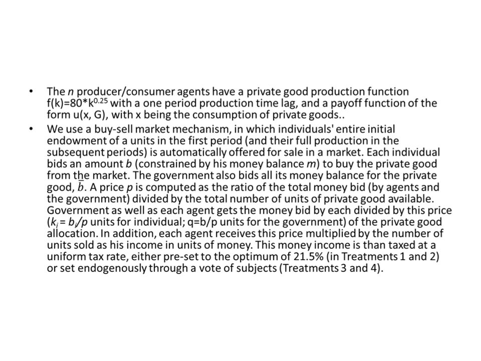
18. Model 1: An Economy with a Generic Public Good In describing the experimental game we minimize the formal notation (see Appendix A for the details). The game has a government and n individual agents each initially endowed with quantity of private good and money (a, m). The government is endowed with G units of the public good and M units of money at the outset. It also has the right to tax a fraction θ of individuals' production of private goods, and a production function that transforms its tax revenues into public goods.

19. The government has as its control parameters an income tax rate θ on the individuals. A move by an agent i in any period t is to decide how much to bid (b ti ) and, after she receives the private good from the market, how much to consume and how much to put into production for the following period. As we set these parameters it is as though we are treating the government as a strategic dummy. Our theory evaluates equilibrium as though the number of agents is large enough that they can be approximated as having no influence over price. For n=10, as used in our experiment, we may expect that some small oligopolistic influence will be present. Even at this level of simplicity, given that production takes time there are accounting questions to be considered in the definition of periodic income and profits. In a stationary equilibrium the timing differences disappear.

20. Experimental Setup 10 subjects in identical situation There is money and two kinds of goods in the economy The private good produced, sold, bought and consumed by the participating subjects; some the private good is also bought by the government and used to produce the public good. The public good (e.g., a public facility) which depreciates at the rate of 10 percent per round. The government uses tax collected from subjects to replenish the depreciating stock of public good. Each subject initially endowed with quantity of private good and money (a, m) = (217, 4700). Private good production function is: UNITS OF THE PRIVATE GOOD PRODUCED = 80*(UNITS INVESTED) 0.25

21. Experimental Setup The government is endowed with G=427 units of the public good and M = 13,000 units of money at the outset. It also has the right to tax a fraction θ of individuals' production of private goods, and a public good production function that transforms its tax revenues into public goods: UNITS OF THE PUBLIC GOOD PRODUCED = 2*(UNITS OF PRIVATE GOOD INVESTED) 0.5 Public good stock depreciates by 10 percent each period Production of public good is added to the stock

22. Market Structure Sell-all minimal market structure: All money in the hands of the 10 agents (47,000 in period 1) and government (13,000 in period 1) is pooled and divided by all units in the hands of the 10 agents (2170 in period 1) to determine the price (27.65 in period 1) Allocations to 10 agents (170 units of good and 6,000 units of money in period 1) and government (13,000/27.65 units of private good in period 1) Government collects taxes at rate theta on money income of agents Agents divide their allocation of good between consumption and production of private good for the next period UNITS OF THE PRIVATE GOOD PRODUCED = 80*(UNITS INVESTED) 0.25 Government converts its share of private goods to produce public goods: UNITS OF THE PUBLIC GOOD PRODUCED = 2*(UNITS OF PRIVATE GOOD INVESTED) 0.5 Perod payoff of agents = private good consumed +public good stock/4 Money is just medium of exchange, has no other role in the economy

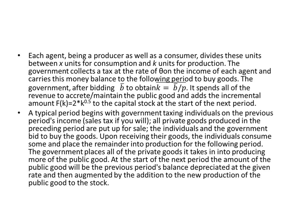
25. In equilibrium this precisely covers depreciation, otherwise the amount of capital stock changes. This describes one full period of the game. If the game ends at period T we must specify terminal or “salvage value” conditions for left over money, goods and the public good. For formal completeness we require salvage values, although in general we have noted that in many experiments the inclusion of a discount βseems to have little influence on play until a few periods near the very end of the sessions. Out of equilibrium there could be degradation or improvement to the public good. For simplicity we assume that depreciation is a fixed percent of the level of capital stock.

26. Experimental Design for Treatments 1 and 2 The experiment consists of variations on tax rate and initial endowment with public goods in a 2x2 design. The first variation (choice of taxation) takes two values: exogenous fixed tax rate θ = 21.5% and endogenous tax rate determined as the median of proposals from individual agents once every four periods. The second variation (initial level of public goods) also takes two values: optimal (G*) and 50 percent of the optimal. Number of individual agents in the economy (n) = 10 Initial endowments of each individual agent: Private goods (a) = 217 units Money (m) = 4700 units The single period utility function of individual agents (u(x,G)) = x+G/4 The session payoff function for the individual \[U=\sum_{t=1}^{T}(x_{t}+G_{t})+????]\] Initial endowments of the government Money () = 13000 units Public goods (G) = 427 units in Sessions 1 and 3, 213 units in Sessions 2 and 4 Government public good augmentation F(k)= 2*k 0.5 The natural discount rate (β) = 1 The depreciation rate ($\eta$) = 0.1 The terminal conditions are \textbf{...TO COME..}$..$ From spreadsheet calculations we obtain α=1$ indicating that the

27. Stock of Public Good (Figure 1) The top left box in Figure 1 shows the time series of the stocks of public good observed during the four independent sessions of the experimental economy with fixed tax rate (21.5%), starting with the optimal level (427) of the public good in Period 1 (in thin grey lines). The mean of these four paths is shown in a dark thick line, and the general equilibrium prediction is shown in a dark dashed line. Similar conventions are used to depict data in the other boxes of Figure 1 and in other figures. In all four of these sessions, the stock of public good gradually but quite steadily declined over the 26 rounds from the optimal starting level (427) to the range of 350-399 and to an average of 376. The top right box in Figure 1 shows that in four runs of a similar economy with tax rate fixed at the optimal level (21.5%) but starting with 50 percent of the optimal level of public good (213.5), the stock of public good rose steadily from 213.5 to the range of 351-366 and to an average of 360 (with very little variation across the four sessions). In the bottom left box, the six sessions with endogenously determined tax rate starting with optimal level of public good (427), the stock of public good tended to decline over the rounds to the range of 348-398 and to an average of 364. In the bottom right box, the six sessions with endogenously determined tax rates but starting from half the optimal level of public good (213.5), the stock of public good tended to rise to the range of 269-402 and to an average of 340. A comparison of the data in the four boxes of Figure suggests some differences but also some similarities. The stock of public good shows great dispersion across economies when tax rates are endogenous instead of being fixed. Starting from the optimal level, the stock of public good tends to decline to the neighborhood of 370 irrespective to whether the tax rate is fixed or determined by the vote of participants. Similarly, starting from the suboptimal level, the stock of public good tends to rise gradually to the neighborhood of 360 irrespective of whether the tax rate is fixed or determined by the vote of participants. Perhaps it is not unreasonable to infer, on the basis of these 20 independent sessions of the economies that the stock of public good tends towards the range of 350-375, and this range seems to form a domain of attraction for these economies. This domain is below the optimum (427), but even further away from zero, which would also be a possibility.

28. Figure 1: Stock of Public Good in Economies Grouped by Four Types of Sessions

29. Efficiency (Figure 2) Efficiency of these economies is defined as the percent of the total points earned by all subjects as a percent of the number of points they would have earned if the economies had achieved general equilibrium outcomes. Results for the 20 sessions are presented in the four boxes of Figure 2 which parallel the layout of boxes in Figure 1 for stock of public good. With fixed tax rate and optimal start (top left box) efficiencies started close to 100 percent tended to decline gradually, albeit noisily, to the range 67-91 percent and average of 80 percent. With suboptimal start (top right box) efficiencies lie near 80 percent at the beginning and the end of the sessions with little perceptible drift over time. With endogenous tax rates and optimal start (bottom left box) efficiencies remain scattered around the low 90s. Only with endogenous tax rates and suboptimal start (bottom right box) do the efficiencies show a steady rise from low 70s to mid 80s over the 26 rounds. Perhaps it is reasonable to infer that 80-90 percent is the domain of attraction for the efficiency of these economies. Also, efficiency is slightly higher with endogenous choice of tax rate. While the stock of public good and efficiency of these economies are overall measures of their performance, we can also assess the decisions made by subjects that led to these outcomes. In the following paragraphs we present the analysis of the subject decisions.

30. Figure 2: Efficiency of Public Good Economies Grouped for Four Types of Sessions

31. Figure 3: Total Production of Private Good in Economies Grouped by Four Types of Sessions

32. Figure 4: Total Consumption as Percentage of Total Individual Purchases of Private Good in Economies Grouped by Four Types of Sessions

33. Figure 5: Total Consumption as Percentage of General Equilibrium Consumption of Private Good in Economies Grouped by Four Types of Sessions

34. Figure 6: Tax Rates

35. Conclusions We are not there yet!

36. Screen 2

37. History Screen

38. Production Function: UNITS OF THE PRIVATE GOOD PRODUCED = 80*(UNITS INVESTED) 0.25

39. Public Good Production Function: UNITS OF THE PUBLIC GOOD PRODUCED = 2*(UNITS OF PRIVATE GOOD INVESTED) 0.5

40. Payoff Function POINTS = CONSUMPTION OF PRIVATE GOOD + PUBLIC GOOD/4