1. Bob Weigel George Mason University

2.  “We are still in the process of identifying characteristic behavior that identifies various modes as separate phenomena.”  “We do not completely understand the solar wind conditions or internal state of the magnetosphere that allows a particular mode.” From FG13 (Modes of Solar Wind Magnetosphere Energy Transfer) Description:

3.  Response Mode definition and some named magnetosphere response modes  Model and Mode ID using a “System ID” approach  Three examples of Model and Mode ID using SID  Other Mode ID approaches

4.  A type of coupling to the solar wind (depends on different physical energy transfer process )  Unique observational characteristics in a magnetospheric measurement (e.g., a “type” of response). Presumably explainable by solar wind energy transfer process/and magnetosphere preconditioning. Functional definition: Mode ID is used to develop better model of system

5.  Storms  Substorms  Steady Magnetospheric Convection  Sawtooth Injection Events  Poleward Boundary Intensifications  Pseudo-break-ups  HILDCAA  …

6.  Mode definition and some named magnetosphere modes  Model and Mode ID using a “System ID” approach  Three examples of Mode ID using SID  Other Mode ID approaches

8.  Start with data and some physical guidance and derive model structure.  Does model structure reveal mode? This is referred to as “System Identification” in statistics and engineering literature (e.g, Ljung, 1999) (note implicit definition of mode here)

9. a) G(t) = p 0 + p 1 S(t) b) G(t) = p 0 + p 1 S(p,t) c) dG/dt + f 1 (p 1, G) = f 2 (p 2,S(t)) d) G(t) = p 0 + p 1 S(t-1)+…+p T S(t-T) e) G(t) = p’ 0 +p’ 1 S(t-1)+…+p’ T S(t-T) G(t) is an averaged measurement centered on time t and S(t) is an average solar wind measurement centered on time t p represents a vector of free parameters. p’ represents free parameters that depend on another variable. Model structure is represented by p and S

10. 1. Integrate over all time, compute error (prediction efficiency of predicted vs actual). 2. Modify parameter(s) and goto 1.

11. G(1) = p o + p 1 S(0)+p 2 S(-1)+…+p T S(1-T) G(2) = p 0 + p 1 S(1)+p 2 S(0)+…+p T S(2-T) G(3) = p 0 + p 1 S(2)+p 2 S(1)+…+p T S(3-T) G(N) = p 0 +p 1 S(N-1) +p 2 S(N-2)+…+p T S(N-T) … One approach is to solve d) using a “sort” variable, e.g., amplitude of G or N sw in a given time range. OLS – “Ordinary Least Squares” Usually N >> T Bargatze et al., 1985 early example of this. d) e) G(t) = p 0 +p 1 S(t-1) +p 2 S(t-2)+…+p T S(t-T) G(t) = p’ 0 +p’ 1 S(t-1) +p’ 2 S(t-2)+…+p’ T S(t-T)

12. G(1) = p o +p 1 S(0) + … G(2) = p 0 +p 1 S(1)+p 2 S(0) … G(3) = p 0 +p 1 S(2)+p 2 S(2)+p 3 S(0) … G(4) = p 0 +p 1 S(3)+p 2 S(2)+p 3 S(1) +p 4 S(0)… If S(0) = 1 and S(t)=0 otherwise, only p 0 and boxed terms are non-zero Plot of p is usually referred to as an impulse response - shows coefficients and has a dynamical interpretation

13.  Mode definition and some named magnetosphere modes  Model and Mode ID using a “System ID” approach  Three examples of Mode ID using SID 1. ID of MeV response modes 2. Un-ID of a mode 3. ID of N sw mode  Other Mode ID approaches

14. 1. ID of MeV response modes  Assume a model of form d) (impulse response)  Select S(t) that gives best prediction  Model parameter and input dependence on L- shell reveal modes 2. Un-ID of a mode 3. ID of N sw mode

15. L-value

16. Impulse in V sw at t=0 Although main driver is V sw - modes P1 and P0 have different dependence on B z. Compare with Li et al. [2001] diffusion model? Vassiliadis et al., [2003]

17. 1. ID of MeV response modes 2. Un-ID of a mode  Failure of model of form a) inspires search for new mode.  Use of form d) indicates new mode may not be needed 3. ID of N sw mode

18.  Russell and McPherron [1972]: Semiannual variation in geomagnetic activity explained by semiannual variation of effective solar wind input.  Mayaud [1973] – Problem because diurnal (UT) prediction  Cliver [2000] – Problem because of day-of-year amplitude plot (see next slide); Could be angle between V sw and dipole  Newell et al. [2002] – Could be “UV insulation” effect  Russell et al. [2003] – Could be day-of-year variation in reconnection line length effect

19. Blue only predicts about 33% of actual semiannual variation. (0% for AL) (Implied) Model of SW/M-I coupling is: 3-hour average of geomagnetic index = 3-hour average of Bs Is remaining 66% explained by Change in reconnection efficiency? Conductance effects?

20. Weigel [2007] ~66% of variation explained when time history of B s is included. ~75% when solar wind velocity is included In auroral zone, result is 50% of semiannual variation is explained by solar wind (up from 0%) am(t) = p 0 +p 1 B s (t-1)+…+p 24 B s (t-24) am subset where B s available All available am

21. 1. ID of MeV response modes 2. Un-ID of a mode 3. ID of N sw mode  Model c) gives different result than e)

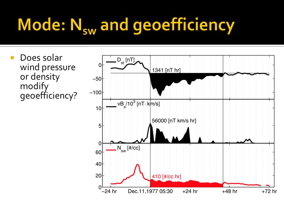
22.  Does solar wind pressure or density modify geoefficiency?

24.  Many studies have looked at modifying input, S(t), in Burton equation  Most recent finding is that modifying S(t) by P dyn 1/2 gives improvement. New mode?  Others have looked at modifying   What if you don ’ t constrain to Burton eqn, but constrain to be linear response? D st (t) = p 0 +p 1 S(t-1)+p 2 S(t-1)+…+p 48 S(t-48)

25. Can repeat with Vsw to argue N sw modifies response efficiency, not P dyn. Weigel [2010] Burton model is constrained to this response function Normalized D st response Time since impulse [hours]

27.  Storms  Substorms  Steady Magnetospheric Convection  Sawtooth Injection Events  Poleward Boundary Intensifications  Pseudo-break-ups  HILDCAA  … See McPherron et al., 1997

28.  Define constraints on magnetospheric conditions  Look for time intervals that satisfy  Quantify solar wind behavior during intervals  Ideally analysis will allow us to say:  under these solar wind conditions, this mode will occur with some probability or  this behavior implies modification of existing model necessary  How do we get here?