Download presentation
Presentation is loading. Please wait.

1
Model Comparison

2
Assessing alternative models We don’t ask “Is the model right or wrong?” We ask “Do the data support a model more than a competing model?” Strength of evidence (support) for a model is relative: Relative to other models: As models improve, support may change. Relative to data at hand: As the data improve, support may change.

3
Assessing alternative models Likelihood ratio tests. Akaike’s Information Criterion (AIC).
.")
4
Recall the Likelihood Axiom “Within the framework of a statistical model, a set of data supports one statistical hypothesis better than other if the likelihood of the first hypothesis, on the data, exceeds the likelihood of the second hypothesis”. (Edwards 1972)
.")
5
Likelihood ratio tests Statistical evidence is only relative, that is, it only applies to one model (hypothesis) in comparison with another. The likelihood ratio L A (x) /L B (x) measures the strength of evidence favoring hypothesis A over hypothesis B. Likelihood ratio tests tell us something about the strength of evidence for one model vs. another. If the ratio is very large, hypothesis A did a much better than B in predicting which value X would take, and the observation X=x is very strong evidence for A versus B. Likelihood ratio tests apply to pairs of hypotheses tested using the same dataset.
 /L B (x) measures the strength of evidence favoring hypothesis A over hypothesis B. Likelihood ratio tests tell us something about the strength of evidence for one model vs. another. If the ratio is very large, hypothesis A did a much better than B in predicting which value X would take, and the observation X=x is very strong evidence for A versus B. Likelihood ratio tests apply to pairs of hypotheses tested using the same dataset..")
6
Likelihood ratio tests Ratios of log-likelihoods (R) follow a chi-square distribution with degrees of freedom equal to the difference in the number of parameters between models A and B.
 follow a chi-square distribution with degrees of freedom equal to the difference in the number of parameters between models A and B.")
7
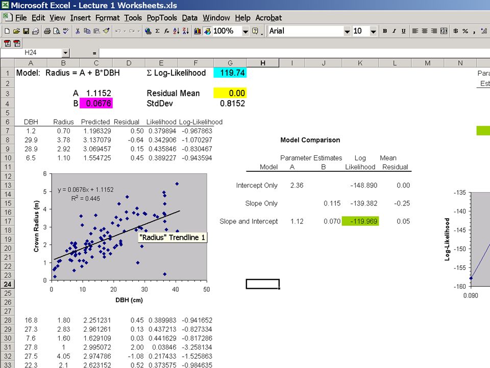
The Data: x i = measurements of DBH on 50 adult trees y i = measurements of crown radius on those trees The Scientific Models: y i = x i + Linear relationship, with 1 parameters ( and an error term ( ). y i = x i + Linear relationship, with 2 parameters ( and an error term ( ). y i = + λ x i 2 + Non-linear relationship with three parameters and an error term ( ). The Probability Model: is normally distributed, with mean = E[X] and variance estimated from the observed variance of the residuals. An example
. y i = + λ x i 2 + Non-linear relationship with three parameters and an error term ( ). The Probability Model: is normally distributed, with mean = E[X] and variance estimated from the observed variance of the residuals. An example.")
8
Procedure 1.Initialize parameter estimates. 2.Using parameter estimation routine, find the parameter values that maximize the likelihood given the model and a normal error structure. 3.Calculate difference in likelihood between models. 4.Conduct likelihood ratio tests. 5.Choose best model of the three candidate models.

9
Remember Parsimony The question is: Is the more complicated model BETTER than the simpler model?

10
Results For model 2 to be better than model 1, twice the difference in likelihoods between the models must be greater than the value of the chi-square distribution with 1 degree of freedom at p = 0.05 χ 2 (df 1) = 3.84 χ 2 (df 2) = 5.99
 = 3.84 χ 2 (df 2) = 5.99")
11
Results Model 2 > Model 3 > Model 1

14
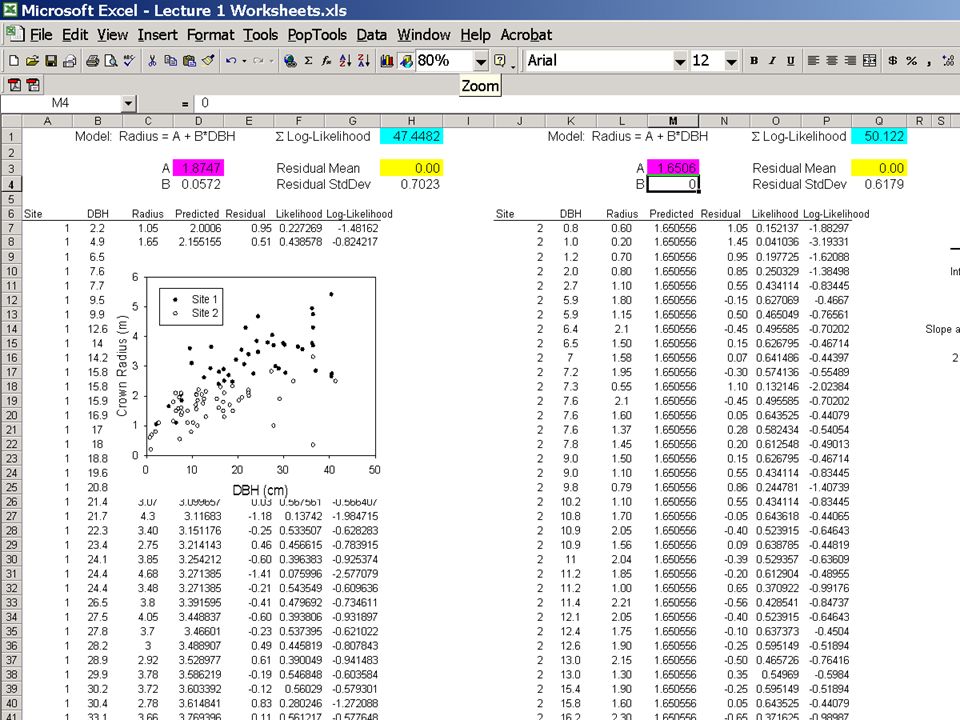
Model comparison Is the two population model better?

15
Model selection when probability distributions differ by model The model selection framework allows error structure to vary over models included in the set of candidate models but….. No component part of the likelihood function can be dropped. Scientific model must remain constant over the models being compared. We must adjust for the different number of parameters in each probability model.

16
An example The Data: x i = measurements of DBH on 50 trees y i = measurements of crown radius on those trees The Scientific Model: y i = x i + [2 parameters ( The Probability Models: is normally distributed, with E[x] predicted by the model and variance estimated from the observed variance of the residuals. is lognormally distributed, with E[x] predicted by the model and variance estimated from the observed variance of the residuals.
![An example The Data: x i = measurements of DBH on 50 trees y i = measurements of crown radius on those trees The Scientific Model: y i = x i + [2 parameters ( The Probability Models: is normally distributed, with E[x] predicted by the model and variance estimated from the observed variance of the residuals.](http://images.slideplayer.com/39/10842417/slides/slide_16.jpg " is lognormally distributed, with E[x] predicted by the model and variance estimated from the observed variance of the residuals..")
17
Back to the example The normal and lognormal have an equal number of parameters so we can compare the likelihoods directly. In this case, the normal probability model is supported by the data.

18
A second example The Data: x i = measurements of DBH on 50 trees. y i = counts of seedlings produced by trees. The Scientific Model: y i = STR*(DBH/30) + exponential relationship, with 1 parameter ( and an error term ( ) The Probability Models: Data follow a Poisson distribution, with E[x and variance = λ Data follow a Negative binomial distribution with E[x =m and variance = m + m 2 /k where k is the clumping parameter.
 + exponential relationship, with 1 parameter ( and an error term ( ) The Probability Models: Data follow a Poisson distribution, with E[x and variance = λ Data follow a Negative binomial distribution with E[x =m and variance = m + m 2 /k where k is the clumping parameter..")
19
Back to the example The binomial requires estimation of one extra parameter, k generally known as the clumping parameter. Thus, twice the difference in likelihoods between the two models must be greater than χ 2 (df 1) = 3.84.
 =")
20
Information theory Information theory Probability Statistics Economics Mathematics Computer Science Physics Communication theory

21
Kullblack-Leibler Information (aka. distance between 2 models) If f(x) denotes reality, we can calculate the Information lost when we use g(x) to approximate reality as: This number is the distance between reality and the model.
 If f(x) denotes reality, we can calculate the Information lost when we use g(x) to approximate reality as: This number is the distance between reality and the model..")
22
Interpretation of Kullblack-Leibler Information (aka. distance between 2 models) Measures the (asymmetric) distance between two models. Minimizing the information lost when using g(x) to approximate f(x) is the same as maximizing the likelihood. 05101520 GAMMA 0 130 260 390 520 650 Count 05101520 WEIBULL 0 130 260 390 520 650 05101520 LOGNORMAL 0 130 260 390 520 650 f(x) g 1 (x) g 2 (x) Truth Approximations to truth
 Measures the (asymmetric) distance between two models. Minimizing the information lost when using g(x) to approximate f(x) is the same as maximizing the likelihood GAMMA Count WEIBULL LOGNORMAL f(x) g 1 (x) g 2 (x) Truth Approximations to truth.")
23
Kullblack-Leibler Information and Truth TRUTH IS A CONSTANT Then, the relative directed distance between truth and model g

24
Interpretation of Kullblack-Leibler Information (aka. distance between 2 models) Minimizing KL is the same as maximizing entropy. We want a model that does not respond to randomness but does respond to information. We maximize entropy subject to the constraints of the model used to capture information in the data. By maximizing entropy, subject to a constraint, we leave only the information supported by the data. The model does not respond to noise
 Minimizing KL is the same as maximizing entropy. We want a model that does not respond to randomness but does respond to information. We maximize entropy subject to the constraints of the model used to capture information in the data. By maximizing entropy, subject to a constraint, we leave only the information supported by the data. The model does not respond to noise.")
25
Akaike’s Information Criterion ^ Akaike defined “an information criterion” that related K-L distance and the maximized log-likelihood as follows: This is an estimate of the expected, relative distance between the fitted model and the unknown true mechanism that generated the observed data. K=number of estimable parameters

26
Information and entropy (noise)
")
27
A refresher on Shannon’s diversity index

28
AIC and statistical entropy

29
Akaike’s Information Criterion ^ AIC has a built in penalty for models with larger numbers of parameters. Provides implicit tradeoff between bias and variance.

30
Akaike’s Information Criterion 1.We select the model with smallest value of AIC. 2.This is the model “closest” to full reality from the set of models considered. 3.Models not in the set are not considered. 4.AIC will select the best model in the set, even if all the models are poor! 5.It is the researcher’s (your) responsibility that the set of candidate models includes well founded, realistic models.
 responsibility that the set of candidate models includes well founded, realistic models..")
31
Akaike’s Information Criterion Estimates the expected, relative distance between the fitted model and the unknown true mechanism that generated the observed data. The best model is the one with the lowest AIC. K = number of estimable parameters ^ Built-in penalty for greater number of parameters.

32
AIC and small samples 1.Unless the sample size (n) is large with respect to the number of estimated parameters (K), use of AIC c is recommended. 2.Generally, you should use AIC c when the ratio of n/K is small (less than 40). 3.Use AIC or AIC c consistently in an analysis rather than mix the two criteria. 4.Use the value of K for the global (most complicated model).
. 3.Use AIC or AIC c consistently in an analysis rather than mix the two criteria. 4.Use the value of K for the global (most complicated model)..")
33
Some Rough Rules of Thumb 1.Differences in AIC (Δ i ’s) can be used to interpret strength of evidence for one model vs. another. 2.A Δ value within 1-2 of the best model has substantial and should be considered along with the best model. 3.A Δ value within 4-7 of the best model has considerably less support. 4.A Δ value > 10 that of the best model has virtually no support and can be omitted from further consideration.

34
Akaike weights Akaike weights (w i ) are considered as the weight of evidence in favor of model i being the actual best model for the situation at hand given that one of the R models must be the best model for that set of R models. where Akaike weights for all set of models considered should add up to 1.

35
Uses of Akaike weights “Probability” that the candidate model is the best model. Relative strength of evidence (evidence ratios). Variable selection—which independent variable has the greatest influence? Model averaging.
. Variable selection—which independent variable has the greatest influence. Model averaging..")
36
An example The Data: x i = measurements of DBH on 50 trees y i = measurements of crown radius on those trees The Scientific Models: y i = x i + [1 parameter ( y i = x i + [2 parameters ( y i = x i + γ x i 2 + [3 parameters ( γ The Probability Model: is normally distributed, with mean = 0 and variance estimated from the observed variance of the residuals...

37
Back to the example Akaike weights can be interpreted as the estimated probability that model i is the best model for the data at hand, given the set of models considered. Weights > 0.90 indicate strong inferences can be made using just that model.

38
Evidence ratios 1.Evidence ratios represent the evidence about fitted models as to which is better in an information sense. 2.These ratios do not depend on the full set of models.

39
Strength of evidence: AIC ratios Very strong evidence that models 2 and 3 are better models than model 1 but the ratio of model 2 to 3 is low suggesting data do not support strong inference.

40
Akaike weights and relative variable importance Estimates of relative importance of predictor variables can be made by summing the w of variables across all the models where the variables occur. Variables can be ranked using these sums. The larger this sum of weights, the more important the variable is.

41
Ambivalence The inability to identify a single best model is not a defect of the AIC method. It is an indication that the data are not adequate to reach strong inference. What is to be done?? MULTIMODEL INFERENCE AND MODEL AVERAGING

42
Strength of evidence: AIC ratios Hard to choose between model 2 and model 3 because of the low value of evidence ratio.

43
Multimodel Inference If one model is clearly the best (w i >0.90) then inference can be made based on this best model. Weak strength of evidence in favor of one model suggests that a different dataset may support one of the alternate models. Designation of a single best model is often unsatisfactory because the “best” model is highly variable. We can compute a weighted estimate of the parameter using Akaike weights.

44
Akaike Weights and Multimodel Inference Estimate parameter values for the two most likely models. Estimate weighted average of parameters across supported models. Only applicable to linear models (Jensen’s ineq). For non-linear models, we can average the predicted response value for given values of the predictor variables.
. For non-linear models, we can average the predicted response value for given values of the predictor variables..")
45
Akaike Weights and Multimodel Inference Estimate of parameter A = (0.73*1.04) +(0.27*1.31)= 1.11 Estimate of parameter B = (0.73*2.1) +(0.27*1.2)= Estimate of parameter C= (0.73*0) +(0.27*3)=
 +(0.27*1.31)= 1.11 Estimate of parameter B = (0.73*2.1) +(0.27*1.2)= Estimate of parameter C= (0.73*0) +(0.27*3)=")
46
Model uncertainty Different datasets are likely to yield different parameter estimates. Variance around parameter estimates is calculated using the dataset at hand and is an underestimate of the true variance because it does not consider model uncertainty. Ideally, inferences should not be limited to one particular dataset. Can we make inferences that are applicable to a larger number of datasets?

47
Techniques to deal with model uncertainty 1.Theoretical: Monte Carlo simulations. 2.Empirical: Bootstrapping Use Akaike weights to calculate unbiased variance for the parameter estimates.

48
Summary: Steps in Model Selection 1.Develop candidate models based on biological knowledge. 2.Take observations (data) relevant to predictions of the model. 3.Use data to obtain MLE of parameters. 4.Evaluate evidence using AIC. 5.Evaluate estimates of parameters relative to direct measurements. Are they reasonable and realistic?
 relevant to predictions of the model. 3.Use data to obtain MLE of parameters. 4.Evaluate evidence using AIC. 5.Evaluate estimates of parameters relative to direct measurements. Are they reasonable and realistic .")
Similar presentations

 Tests>")


