1. Normal Distribution 1

2. Objectives  Learning Objective - To understand the topic on Normal Distribution and its importance in different disciplines.  Performance Objectives At the end of this lecture the student will be able to:  Draw normal distribution curves and calculate the standard score (z score)  Apply the basic knowledge of normal distribution to solve problems.  Interpret the results of the problems. 2

3. Data can be distributed in different ways 3

4. Skewed to L 4

5. 5

6. Normal distribution 6

7. What is Normal Distribution?  It is defined as a continuous frequency distribution of infinite range* (can take any values not just integers as in the case of binomial).  Continuous probability function – real observation will fall between two real limits or numbers  This is the most important probability distribution in statistics and important tool in analysis of epidemiological data and management science. 7

8. What follows normal distribution? 8

9.  Heights of people  BP measurements  Test results 9

10. The normal distribution  symmetric,  bell-shaped Probability X 10

11. 11 Characteristics of the Normal Distribution 1. Has a Bell Shape Curve 2. It is symmetrical about the mean µ. The curve on either side of µ is a mirror image of the other side. 50% of values above mean, 50% below mean 3. The mean, the median and the mode are equal. 4. The total area under the curve above x-axis =1

12. Irwin/McGraw-Hill © The McGraw-Hill Companies, Inc., 1999 -5 0.4 0.3 0.2 0.1.0 x f ( x ral itrbuion:  =0,  = 1 Characteristics of a Normal Distribution Mean, median, and mode are equal Normal curve is symmetrical Theoretically, curve extends to infinity a

13. Effects of  and 

14. Relationship between Standard Deviation and normal distribution 14

15. 15

16. 16

17. 68-95-99.7 Rule 68% of the data 95% of the data 99.7% of the data

18. Example  95% of students are between 1.1m and 1.7m tall.  Assuming data is normally distributed calculate the mean and standard deviation. 18

19.  Mean is half way between 1.1 m and 1.7m  So..Mean = (1.1 + 1.7) /2 = 1.4 m  95% of data is under 2 standard deviations from mean, that is 4 standard deviations give 95% of data  1 standard deviation = 1.7-1.1/4  = 0.6m/4 = 0.15m 19

20. 20

21. Example 2  68% of Blood pressures of girls at JUST are from 100mmHg to 120 mmHg  Assuming normal distribution what is the mean of BP of girls?  What is the standard deviation? 21

22. The Normal Distribution X Changing μ shifts the distribution left or right. Changing σ increases or decreases the spread.

23. Does everything follow a normal distribution?  NO!  We will discuss this more when looking at central limit theorem.  Normal distribution is a very and perhaps most useful concept in statistics! But you can only apply these rules if the distribution is normal. 23

24. Which of these would have a normal distribution?  Shoe size  Income in Jordan  Fasting sugar levels in a population  Number of cigarettes smoked per person  But central limit theorem can make something with random distribution approximate a normal distribution. 24

25. How can we compare many normal distributions?  If a data set has a normal distribution we can use it and compare it to other datasets with a normal distribution 25

26. Standard normal distribution  This makes all normal distributions comparable, by dividing their distribution by the standard deviation.  The standard score, sigma or z score is the number of standard deviations from the mean 26

27. Characteristics of Normal Distribution Cont’d  Hence Mean = Median = Mode  The total area under the curve is 1 (or 100%)  Normal Distribution has the same shape as Standard Normal Distribution.  In a Standard Normal Distribution: The mean (μ ) = 0 and Standard deviation (σ) =1 27

28. The Standard Normal Distribution A normal distribution with a mean of 0 and a standard deviation of 1 is called the standard normal distribution. Z value: The distance between a selected value, designated X, and the population mean, divided by the population standard deviation, 28

29. Comparing X and Z units Z 100 2.00 200X (  = 100,  = 50) (  = 0,  = 1)

30. Z Score  Z = X - μ  Z indicates how many standard deviations away from the mean the point x lies.  Z score is calculated to 2 decimal places. σ 30

31. Why use z-scores? 1. z-scores make it easier to compare scores from distributions using different scales. e.g. two tests: Test A: Fred scores 78. Mean score = 70, SD = 8. Test B: Fred scores 78. Mean score = 66, SD = 6. Did Fred do better or worse on the second test?

32. Test A: as a z-score, z = (78-70) / 8 = 1.00 Test B: as a z-score, z = (78 - 66) / 6 = 2.00 Conclusion: Fred did much better on Test B.

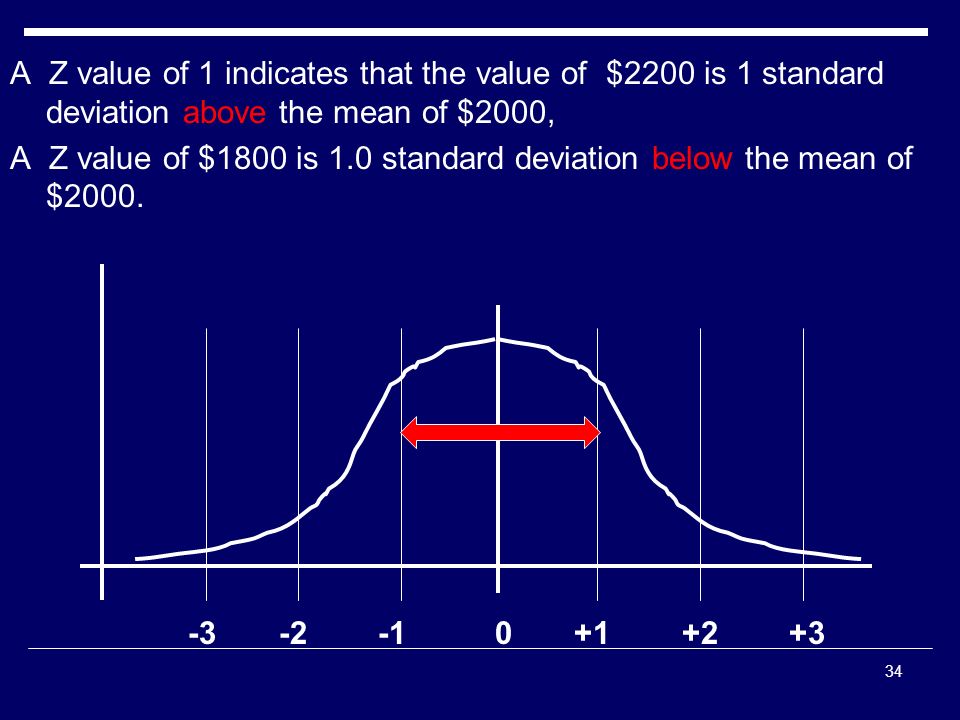
33. EXAMPLE The monthly incomes of recent MBA graduates in a large corporation are normally distributed with a mean of $2000 and a standard deviation of $200. What is the Z value for an income of $2200? And an income of $1800? For X=$2200, Z=(2200-2000)/200= 1.0 For X=$1800, Z =(1800-2000)/200= -1.0 What does that mean????? 7-7 33

34. 34 A Z value of 1 indicates that the value of $2200 is 1 standard deviation above the mean of $2000, A Z value of $1800 is 1.0 standard deviation below the mean of $2000. -3 -2 -1 0 +1 +2 +3

35. Looking up probabilities in the standard normal table What is the area to the left of Z=1.51 in a standard normal curve? Z=1.5 1 Area is 93.45%

36. Tables  Areas under the standard normal curve (Appendices of the textbook) 36

37. 37

38. 38

39. 39

40. Distinguishing Features  The mean ± 1 standard deviation covers 66.7% of the area under the curve  The mean ± 2 standard deviation covers 95% of the area under the curve  The mean ± 3 standard deviation covers 99.7% of the area under the curve 40

41. Distinguishing Features

42. 68-95-99.7 Rule 68% of the data 95% of the data 99.7% of the data

43. Exercises  Assuming the normal heart rate (H.R) in normal healthy individuals is normally distributed with Mean = 70 and Standard Deviation =10 beats/min 43

44. Exercise # 1 Then: What area under the curve is under 80 beats/min? And what area under the curve is above 80 beats/min? Now we know, Z =X-M/SD Z=? X=80, M= 70, SD=10. So we have to find the value of Z. For this we need to draw the figure…..and find the area which corresponds to Z. Z=1 then one SD above the mean. 44

45. Exercise # 1 0.159 The value of z from the table for z=1.00 is 0.8413. So 84% have heart rate of 80 beat s or less per minute. Then 1 - 0.8413= 0.159. This means that 15.9% of individuals have a heart rate above one standard deviation (greater than 80 beats per minute). 0.8413 Z score 45 -3 -2 -1 μ 1 2 3

46. Exercise # 2 Then: 2) What area of the curve is below 90 beats/min? And what are of the curve is above 90 beats/min? 46

47. -3 -2 -1 μ 1 2 3 Diagram of Exercise # 2 0.023 47 Solution: Find Z score then for x=90 Then look at the table. Z = 2 Area below 2 = 0.9772 and area above 2 = 1- 0.9772 = 0.023

48. Exercise # 3 Then: 3) What area of the curve is between 50-90 beats/min? 48

49. -3 -2 -1 μ 1 2 3 Diagram of Exercise # 3 0.954 49

50. Exercise # 4 Then: 4) What area of the curve is above 100 beats/min? 50

51. -3 -2 -1 μ 1 2 3 Diagram of Exercise # 4 0.015 51

52. Exercise # 5 5) What area of the curve is below 40 beats per min or above 100 beats per min? 52

53. Diagram of Exercise # 5 0.015 53 -3 -2 -1 μ 1 2 3

54. 54 Example 2 Given the standard normal distribution, find P( z ≥ -1.48) Solution: P ( z ≥ -1.48)= 1- P ( z ≤ -1.48) = 1- 0.0694 = 0.9306

55. 55 Example 3 What proportion of z values are between -1.65 and 1.65 Solution: P (-1.65 ≤ z ≤1.65) = 0.9505 – 0.0495 =0.9010

56. 56 Normal Distribution Application  If the distribution is standard normal distribution with mean of 0 and a standard deviation of 1, we can use table D in appendix of Daniel book and find area under value of z.  Normal distribution is easily to be transformed in to the standard normal distribution through transfer values of X to corresponding values of z.  This is done by using the following formula: Z = x - µ σ

57. Application/Uses of Normal Distribution  It’s application goes beyond describing distributions  It is used by researchers and modelers.  The major use of normal distribution is the role it plays in statistical inference.  The z score along with the t –score, chi-square and F- statistics is important in hypothesis testing.  It helps managers/management make decisions. 57

58. Are my data “normal”?  Not all continuous random variables are normally distributed!!  It is important to evaluate how well the data are approximated by a normal distribution

59. Are my data normally distributed? 1.Look at the histogram! Does it appear bell shaped? 2.Compute descriptive summary measures— are mean, median, and mode similar? 3.Do 2/3 of observations lie within 1 std dev of the mean? Do 95% of observations lie within 2 std dev of the mean? 4.??? 5.???

60. Do it your self 60

61. Example The daily water usage per person in New Providence, New Jersey is normally distributed with a mean of 20 gallons and a standard deviation of 5 gallons. About 68% of the daily water usage per person in New Providence lies between what two values?  That is, about 68% of the daily water usage will lie between 15 and 25 gallons. 61

62. Example What is the probability that a person from New Providence selected at random will use less than 20 gallons per day? The associated Z value is Z=(20-20)/5=0. Thus, P(X<20)=P(Z<0)= 0.5 = 50% What percent uses between 20 and 24 gallons? The Z value associated with X=20 is Z=0 and with X=24, Z=(24-20)/5=.8. Thus, P(20<X<24)=P(0<Z<.8)=28.81% 62

63. Irwin/McGraw-Hill © The McGraw-Hill Companies, Inc., 1999 -5 0.4 0.3 0.2 0.1.0 x f ( x ral itrbuion:  =0, -4 -3 -2 -1 0 1 2 3 4 P(0<Z<.8) =.2881 EXAMPLE 3 0<Z<0.8

64. Calculating z-scores Birthweights at a certain hospital are normally distributed with mean = 112 oz and standard deviation = 21 oz. What is the z-score for an infant with birthweight = 154 oz.? How many standard deviations above the mean is this birthweight? ______ How many standard deviations below the mean is a birthweight of 91 oz? _____

65. Normal Distribution Probabilities What if you want to find the probability that a birthweight is Greater than 9 lbs (144 oz)? Less than 6 lbs (96 oz)? Between 7 lbs (112 oz) and 8 obs (128 oz)?