1. Chapter 10 Comparing Two Populations or Groups Sect 10.1 Comparing two proportions

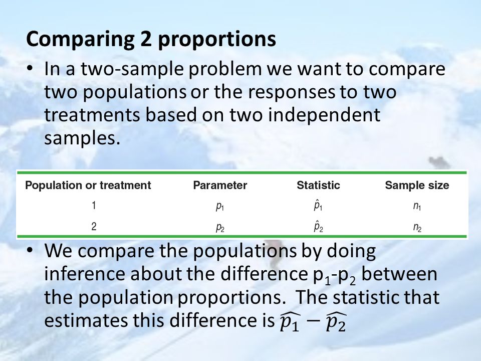
2. A two-sample problem can arise from a randomized comparative experiment that randomly divides subjects into two groups and exposes each group to a different treatment. Comparing random samples separately selected from two populations is also a two- sample problem. Unlike the matched pairs design, there is no matching of the units in the two samples and the two samples can be of different sizes. – This is usually the biggest hint that it’s 2-sample

4. Random: We must have 2 SRSs from the populations of interest. Independent: check n*10< population for each sample Normal: need to check np>10 and nq>10 for each sample

5. Remember: for any two independent random variables X and Y:

6. Example: Who Does More Homework? Suppose that there are two large high schools, each with more than 2000 students, in a certain town. At School 1, 70% of students did their homework last night. Only 50% of the students at School 2 did their homework last night. The counselor at School 1 takes an SRS of 100 students and records the proportion that did homework. School 2’s counselor takes an SRS of 200 students and records the proportion that did homework. School 1’s counselor and School 2’s counselor meet to discuss the results of their homework surveys. After the meeting, they both report to their principals that

9. Confidence Intervals for p 1 – p 2

10. Two-Sample z Interval for a Difference Between Proportions

11. Example: Teens and Adults on Social Networks As part of the Pew Internet and American Life Project, researchers conducted two surveys in late 2009. The first survey asked a random sample of 800 U.S. teens about their use of social media and the Internet. A second survey posed similar questions to a random sample of 2253 U.S. adults. In these two studies, 73% of teens and 47% of adults said that they use social- networking sites. Use these results to construct and interpret a 95% confidence interval for the difference between the proportion of all U.S. teens and adults who use social-networking sites.

12. Plan: We should use a two-sample z interval for p 1 – p 2 if the conditions are satisfied. Random The data come from a random sample of 800 U.S. teens and a separate random sample of 2253 U.S. adults. Normal We check the counts of “successes” and “failures” and note the Normal condition is met since they are all at least 10: Independent We clearly have two independent samples—one of teens and one of adults. Individual responses in the two samples also have to be independent. The researchers are sampling without replacement, so we check the 10% condition: there are at least 10(800) = 8000 U.S. teens and at least 10(2253) = 22,530 U.S. adults. State: Our parameters of interest are p 1 = the proportion of all U.S. teens who use social networking sites and p 2 = the proportion of all U.S. adults who use social-networking sites. We want to estimate the difference p 1 – p 2 at a 95% confidence level.

13. Do: Since the conditions are satisfied, we can construct a two- sample z interval for the difference p 1 – p 2. Conclude: We are 95% confident that the interval from 0.223 to 0.297 captures the true difference in the proportion of all U.S. teens and adults who use social-networking sites. This interval suggests that more teens than adults in the United States engage in social networking by between 22.3 and 29.7 percentage points.

14. Significance Tests for p 1 – p 2 H 0 : p 1 - p 2 = 0 or, alternatively, H 0 : p 1 = p 2 The alternative hypothesis says what kind of difference we expect. H a : p 1 - p 2 > 0, H a : p 1 - p 2 < 0, or H a : p 1 - p 2 ≠ 0 If the Random, Normal, and Independent conditions are met (same as before for confidence intervals) we can proceed with calculations.

15. If H 0 : p 1 = p 2 is true, the two parameters are the same. We call their common value p. But now we need a way to estimate p, so it makes sense to combine the data from the two samples. This pooled (or combined) sample proportion is:

16. Example: Hungry Children Researchers designed a survey to compare the proportions of children who come to school without eating breakfast in two low-income elementary schools. An SRS of 80 students from School 1 found that 19 had not eaten breakfast. At School 2, an SRS of 150 students included 26 who had not had breakfast. More than 1500 students attend each school. Do these data give convincing evidence of a difference in the population proportions? Carry out a significance test at the α = 0.05 level to support your answer. State: Our hypotheses are H 0 : p 1 - p 2 = 0 H a : p 1 - p 2 ≠ 0 where p 1 = the true proportion of students at School 1 who did not eat breakfast, and p 2 = the true proportion of students at School 2 who did not eat breakfast.

17. Plan: We should perform a two-sample z test for p 1 – p 2 if the conditions are satisfied. Random The data were produced using two simple random samples—of 80 students from School 1 and 150 students from School 2. Normal We check the counts of “successes” and “failures” and note the Normal condition is met since they are all at least 10: Independent We clearly have two independent samples—one from each school. Individual responses in the two samples also have to be independent. The researchers are sampling without replacement, so we check the 10% condition: there are at least 10(80) = 800 students at School 1 and at least 10(150) = 1500 students at School 2.

18. Do: Since the conditions are satisfied, we can perform a two-sample z test for the difference p 1 – p 2. P-value Using Table A or normalcdf, the desired P-value is 2P(z ≥ 1.17) = 2(1 - 0.8790) = 0.2420. Conclude: Since our P-value, 0.2420, is greater than the chosen significance level of α = 0.05,we fail to reject H 0. There is not sufficient evidence to conclude that the proportions of students at the two schools who didn’t eat breakfast are different.

19. Example: Significance Test in an Experiment High levels of cholesterol in the blood are associated with higher risk of heart attacks. Will using a drug to lower blood cholesterol reduce heart attacks? The Helsinki Heart Study recruited middle- aged men with high cholesterol but no history of other serious medical problems to investigate this question. The volunteer subjects were assigned at random to one of two treatments: 2051 men took the drug gemfibrozil to reduce their cholesterol levels, and a control group of 2030 men took a placebo. During the next five years, 56 men in the gemfibrozil group and 84 men in the placebo group had heart attacks. Is the apparent benefit of gemfibrozil statistically significant? Perform an appropriate test to find out.

20. State: Our hypotheses are H 0 : p 1 - p 2 = 0ORH 0 : p 1 = p 2 H a : p 1 - p 2 < 0H a : p 1 < p 2 where p 1 is the actual heart attack rate for middle-aged men like the ones in this study who take gemfibrozil, and p 2 is the actual heart attack rate for middle-aged men like the ones in this study who take only a placebo. Note: we are using a small significance level, α = 0.01 to reduce the risk of making a Type I error (concluding that gemfibrozil reduces heart attack risk when it actually doesn’t). Plan: We should perform a two-sample z test for p 1 – p 2 if the conditions are satisfied. Random The data come from two groups in a randomized experiment Normal The number of successes (heart attacks!) and failures in the two groups are 56, 1995, 84, and 1946. These are all at least 10, so the Normal condition is met. Independent Due to the random assignment, these two groups of men can be viewed as independent. Individual observations in each group should also be independent: knowing whether one subject has a heart attack gives no information about whether another subject does.

21. Do: Since the conditions are satisfied, we can perform a two-sample z test for the difference p 1 – p 2. Conclude: Since the P-value, 0.0068, is less than 0.01, the results are statistically significant at the α = 0.01 level. We can reject H 0 and conclude that there is convincing evidence of a lower heart attack rate for middle- aged men like these who take gemfibrozil than for those who take only a placebo. P-value Using Table A or normalcdf, the desired P-value is 0.0068